


Pole-Zero Cancellation
What is Pole Zero Cancellation? | Pole-Zero Cancellation Principles | Single-pole Cancellation | Secondary Factors in Real Amplifiers
Dual-Pole Cancellation | Setting Up Pole-Zero Cancellation
Pole-zero cancellation is an important part of radiation spectroscopy analysis. Converting charges created from radiation events, such as gamma rays produced in gamma spectroscopy, into binnable signals introduces a shaping error which can impact later analysis. This error takes the form of an overcorrection, with the pulse dipping below the zero line. Pole-zero cancellation compensates for this error. However, this must be done carefully though, as overcompensation or under compensation can lead to significant cumulative errors.

Analogue and digital processing systems have different approaches to pole-zero cancellation. In analog radiation spectroscopy systems, this correction is achieved using physical components, namely a resistor in parallel with differentiating capacitor. In digital pulse processing, a deconvolution algorithm is applied to the signal.
In standard analogue systems, this cancellation is done manually, using an oscilloscope to adjust the correction until it visually appears flat. However, in real detector systems and amplifiers, there may be weak secondary poles that cannot be easily identified by eye, yet can introduce non-negligible errors in pulse height measurement or baseline drift at high count rates. To zero these poles requires advanced mathematical processing.
What is Pole Zero Cancellation?
A gamma ray deposits its energy inside a detector crystal, and the generated charge is collected within a few hundred nanoseconds. The resulting signal from a charge-sensitive preamplifier can last up to hundreds of microseconds, often a thousand times longer than the initial event. At higher count rates exceeding a few tens of kilohertz, subsequent pulses systematically pile up on the decay tails of preceding events.
Shaping amplifiers solve this using high-pass filtering, shortening the exponential tail to facilitate rapid baseline recovery. However, this filtering introduces a broad, shallow undershoot where the output signal falls below then rises towards the baseline. This is only a small deviation in each measurement but systematically distorts subsequent pulse amplitude measurements. This impact will increase with each subsequent measurement leading to significant deviations.
Pole-zero cancellation is the standard compensation technique for this. It introduces a specific DC response to the filter network, eliminating the undershoot. This is implemented via a single resistor in analog systems or a single line of digital deconvolution code.
While theoretical preamplifier models assume a single-exponential decay, physical hardware deviates from this ideal. Microscopic stray capacitances, multi-stage electronics, and slow charge collection cause real pulses to decay across multiple timescales. On a standard oscilloscope display, these secondary tails are almost impossible to see. However, at count rates above ~20 kcps, an uncompensated second pole can significantly degrade energy resolution.
Pole-Zero Cancellation Principles
Poles and Zeros
When a charged capacitor discharges through a resistor, the voltage decays exponentially according to:

Where the time constant is τ=RC.
Analyzing multistage circuits in the time domain requires solving systems of differential equations. The Laplace transform simplifies this by representing signals in the form est where s is a generalized complex frequency that describes oscillation, growth, and decay. In the s-domain, differentiation leads to multiplication by s, and integration translates to division by s. Either of these will reduce the complex differential equations to standard algebraic expressions.
This transformation yields the transfer function, H(s), defined as the ratio of the output signal to the input signal as a function of s. For passive resistor-capacitor (RC) networks, this function is always a rational fraction.
Consider a basic low-pass filter consisting of a resistor in series with a capacitor, with the output measured across the capacitor. Because a capacitor has an impedance of 1/sC, the circuit operates as a frequency-dependent voltage divider:

The denominator of this transfer function equals zero at s=-1/RC. This root is known as a pole.
In the time domain, a pole at s=-1/τ corresponds directly to an exponential decay of e-t/τ. Therefore for low pass filters, the magnitude of the pole dictates the decay rate, so a pole located further from the origin along the real axis results in a faster exponential decay.
Reconfiguring the circuit to measure the output across the resistor forms a high-pass filter. The transfer function changes only in its numerator:

The denominator retains the pole at s=-1/RC, preserving the characteristic decay time, τ=RC. However, the numerator now evaluates to zero at s=0. A root of the numerator in a transfer function is called a zero.
A frequency of s=0 corresponds to no oscillation, i.e. a direct current (DC). Therefore, a zero at s=0 indicates that the circuit has zero gain at DC. This is the defining characteristic of a high-pass filter. This total attenuation at DC is the fundamental cause of pulse undershoot.
When consecutive filter stages are used, their combined transfer function is the product of their individual transfer functions, allowing poles and zeros to accumulate algebraically. If an initial stage introduces a pole at s=-1/τ, then a later stage introduces a zero at the same s=-1/τ, the mathematical factor (s+1/τ) appears in both the numerator and denominator. These terms cancel, effectively removing this exponential decay from the final output signal.

Core principles of pole-zero analysis:
- A pole represents an exponential decay, with its distance to the left of the imaginary axis determining the decay rate.
- A zero mathematically overlapping a pole cancels that specific exponential decay.
- A zero at s=0 completely attenuates DC signals, leaving only the dynamic signal components on a zero baseline.
Origin of the exponential tail
A charge-sensitive amplifier integrates the detector’s charge burst Q onto a feedback capacitor Cf, causing the output voltage to rise by Q/Cf. A feedback resistor Rf subsequently drains this capacitor, resulting in a step that decays with a time constant τ=RfCf. Decay times of tens to hundreds of microseconds are typical in these systems.
This decay is deliberately extended for two primary reasons. First, the mean-square Johnson noise current density of Rf is 4kT/Rf. Therefore, maximizing this resistance value minimizes thermal noise contributions. Second, the decay time must significantly outlast the charge collection process within the detector. If the decay is too fast, the measured amplitude becomes dependent on the interaction location within the crystal, (also known as ballistic deficit).

This extended τ inherently causes baseline accumulation. Successive incoming pulses land on the decaying tails of earlier events, transforming the amplifier output into a randomized voltage staircase. Subsequent downstream signal processing must isolate and eliminate this baseline history before individual pulse heights can be measured reliably.
Reset-type preamplifiers bypass this accumulation by omitting Rf entirely and periodically discharging the capacitor using a switch. While this architecture eliminates the exponential tail, it introduces distinct dead-time characteristics. Consequently, many systems currently in service utilize resistive feedback and inherently produce an exponential tail.
Differentiation and the undershoot
These extended tails must be truncated before successive pulses accumulate. Analog shaping achieves this using a differentiator, namely the CR high-pass filter described above, with a time constant τd=RdC, where Rd and C are its resistor and capacitor. This high-pass stage terminates each pulse to ensure subsequent events originate from a stable baseline.
Processing the amplifier’s single-exponential output through this filter yields a dual-exponential response. Assuming τ is much larger than τd,

The first term is the desired shaped pulse. The second term constitutes an undershoot of opposite polarity. This undershoot has a fractional depth of τd/τ and decays according to the primary amplifier time constant. For typical values, such as τd=2 µs and τ=50 µs, the undershoot reaches 4% of the peak amplitude and persists for several hundreds of microseconds, presenting as a shallow but exceptionally wide baseline depression.
Optimizing component values cannot eliminate this artifact, as the high-pass filter possesses a zero at s=0. It inherently has no DC response so the integral of the output signal (i.e. its total area) must equal zero. The area of the undershoot must perfectly balance the area of the positive pulse. Altering component values merely shifts the geometry of this artifact, trading a deep, brief undershoot for a shallow, prolonged one.
Any effective correction must introduce a finite DC response to the circuit.

Single-pole cancellation
Analog Systems
Nowlin and Blankenship published the standard solution to this undershoot in 1965. The analog implementation involves adding an adjustable resistor, RC, in parallel with the differentiating capacitor, C. This configuration introduces a zero at s=-1/(RCC). By calibrating the network such that RCC=RfCf, this zero is positioned exactly over the amplifier’s pole, effectively cancelling it.
Adding this resistor shifts the zero away from the origin. Subsequently, the circuit no longer completely blocks DC signals. At the match point, its DC gain is τd/( τd+τ), or approximately τd/ τ when the shaping time is short compared with the amplifier decay. This finite DC response is sufficient to transmit the total pulse area through the network, eliminating the mathematical requirement for a compensating undershoot. That gain is also the fractional depth of the undershoot it removes. The area the undershoot previously had to supply is exactly the area the DC path now passes.
Digital Systems
Digital shapers achieve this same compensation arithmetically. Accompanying the trapezoidal filter is a single-step deconvolution algorithm:

In this recursion, x(n) represents the incoming digitized sample at index n, and y(n) is the corrected output sample. The decay factor p=e-Ts/τ defines the fraction of the exponential remaining after one sampling period Ts. For high sampling rates, this value approaches unity. It is the sampled-data counterpart of the pole at s=-1/τ, so subtracting p times the previous sample removes exactly the decay that pole represents, in the same way the analog zero does. The factor A is the amplitude of the fitted exponential in ADC counts. Dividing by it sets the recovered step to unit height, so a pulse that produced an amplitude of A at the preamplifier emerges from the filter as a step of one. The absolute value of this gain factor is generally non-critical, as the overall system gain is absorbed during subsequent energy calibration. In the configuration settings of a multichannel analyzer, τ is typically parameterized as the decay time or pole-zero setting.
Because reversing an exponential decay is mathematically equivalent to integration, this digital filter inherently possesses infinite DC gain. The recursion carries the whole of the previous output forward through the y(n-1) term, making it a running sum, so rounding errors and input offsets accumulate indefinitely and eventually drive the output to saturation. Practical firmware implementations mitigate this by applying a slight constant correction to each sample, gradually bleeding the accumulator back toward zero. This baseline restoration mechanism is suspended while an event is actively being measured.
Secondary Factors in Real Amplifiers
A single exponential decay is only a first-order approximation of a physical amplifier’s output. Additional time constants are introduced through several mechanisms:
-
Imperfect Internal Cancellation
Certain preamplifier designs use a deliberately slow initial stage to mitigate ballistic deficit, cancelling that pole in a second stage and substituting a faster one. This deliberate pole-zero pair in the signal path relies on precise component matching, typically via a manually adjusted compensation resistor, RC. Any initial calibration mismatch leaves a residual exponential tail. Also, component values drift with temperature and aging, degrading an initially perfect match over time.
-
Stray capacitance
The physically large feedback resistor has intrinsic stray parasitic capacitance. High-voltage bias decoupling and AC coupling networks downstream contribute additional capacitive effects.
-
Detector effects
Slow charge collection and charge trapping within the detector crystal produce signal tails that mathematically mimic circuit poles, despite lacking a discrete circuit equivalent.
A more accurate model of the preamplifier output is a sum of two exponentials.

In this model, A1 and A2 are the respective amplitudes of the two decay components, while τ1 and τ2 are their associated time constants. The primary component is the decay treated as a single exponential above, so τ1 plays the role of τ and A1 the role of A.
Can You Remove These Undershoots Manually?
The secondary term is usually very small so it cannot be identified by eye. For instance, a published measurement of a germanium detector characterized a primary pole at τ1=49.31 µs containing nearly all the signal amplitude, accompanied by a secondary component comprising approximately 3% of the amplitude with τ2=259.41 µs. A standard single-exponential fit applied to the same empirical data yielded a decay time of 52.77 µs, which appeared statistically sound despite failing to capture the secondary tail.
A 3% amplitude deviation distributed across a quarter of a millisecond is almost impossible to see on a standard oscilloscope. In the referenced study, the authors manually trimmed an amplifier via an oscilloscope as meticulously as possible. However, subsequent mathematical fitting of the captured pulses revealed the system was still improperly compensated.
This highlights the practical weakness of visual scope trimming. The procedure optimizes the visible residual on an isolated pulse, while the residual tail that actively limits energy resolution at high count rates remains obscured below the display’s noise floor.

Measured effect on energy resolution
The same study quantified the spectral cost of an uncompensated secondary pole. Using a Cobalt-60 source at 100 kcps, two-pole compensation improved the 1.33 MeV line from 4.9 keV to 4.0 keV FWHM, and its full-width at tenth-maximum (FWTM) from 10.9 keV to 8.5 keV. Expressed relative to the two-pole result, as the source does, those are gains of 22.5% and 28.2%.
The observation that the tenth-maximum width improves by a larger margin than the half-maximum width is characteristic of low-energy tailing mitigation. Furthermore, FWTM serves as the more sensitive diagnostic metric for identifying residual poles.
Two critical dependencies govern these performance gains:
- Count rate dependence: At low event rates, exponential tails rarely overlap, causing the one- and two-pole methods to perform almost identically. The performance disparity scales directly with count rate.
- Initial analog adjustment: The degree of improvement relies heavily on the baseline accuracy of the physical preamplifier trim. When the same two-pole algorithm was applied to a different crystal in a different detector, the FWHM improvement was only roughly 3% at 55 kcps, compared to the ~22% seen on the previous unit at 100 kcps.
Two-pole digital compensation mathematically recovers the energy resolution lost to imperfect and drifting analog adjustments. While it offers marginal benefits on a system that already works, its practical value lies in eliminating the need to hand-trim and continuously maintain thousands of individual hardware channels as components age.

Dual-Pole Cancellation
Extending the algorithm to two poles requires the introduction of a second zero. Using the parameters A1, A2, τ1, and τ2 derived from the two-exponential fit, a distinct decay factor is defined for each component, one for the pole at s=-1/τ1 and one for the pole at s=-1/τ2:

The resulting digital recursion is expressed as:

The five operational constants are derived from the fitted parameters as follows:
- k1 = 1/(A1+A2)
- k2 = k1(p1+p2)
- k3 = k1p1p2
- k4 = k1[A1(1+p2)+A2(1+p1)]
- k5 = k1(A1p2+A2p1)
The three input terms are not independent. They are what results from applying the single-pole subtraction twice, once for each decay constant.
First this algorithm removes the τ1 component with x(n)-p1x(n-1), then removes the τ2 component from that result. Multiplying the two operations out gives the x(n), x(n-1), and x(n-2) terms above, so the recursion contributes one zero per pole, exactly as two cascaded analog stages would. Setting A2=p2=0 mathematically collapses the function back into the single-pole recursion, allowing a single software architecture to handle both implementations seamlessly. Furthermore, the identity k4-k5=1 holds exactly, providing a reliable mathematical verification for the calculated coefficients.
Further Resources
 ADC Differential and Integral Non-Linearity
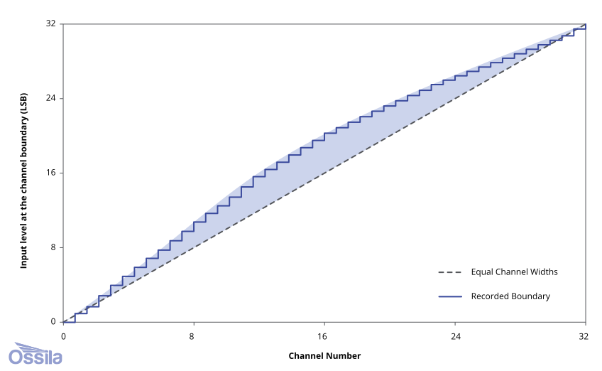
Differential nonlinearity and integral nonlinearity are the two specifications that determine whether an analogue-to-digital converter (ADC) is suited to pulse height spectroscopy. Both usually appear on an ADC’s datasheet.
Read more...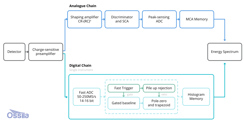 Digital Pulse Processors
In pulse-mode radiation spectroscopy, each electrical pulse carries information about the energy deposited by the quantum of radiation that produced it, proportional to its amplitude. By accurately processing this signal, you can extract information about the energy of that photon or particle.
Read more...Contributors
Written by
Product Developer
Diagrams by
Graphic Designer
References
- Elimination of undesirable undershoot in the operation and..., C. H. Nowlin and J. L. Blankenship, Rev. Sci. Instrum (1965)
- One- and two-pole compensation of charge-sensitive amplifiers with..., T. Stezelberger and S. Zimmermann, IEEE Trans. Nucl. Sci (2023)
- Digital synthesis of pulse shapes in real time..., V. T. Jordanov and G. F. Knoll, Nucl. Instrum. Methods A (1994)
- Radiation Detection and Measurement, G. F. Knoll, Wiley
- Practical Gamma-ray Spectrometry, G. Gilmore, Wiley (2008)