


Digital Pulse Processors
How Do Digital Pulse Processors Work | Analog Systems | Trapezoidal Filter | DPP Components Status | Troubleshooting DPP Systems
In pulse-mode radiation spectroscopy, each electrical pulse carries information about the energy deposited by the quantum of radiation that produced it, proportional to its amplitude. By accurately processing this signal, you can extract information about the energy of that photon or particle.
One primary engineering challenge in this process is due to the random nature of these events. Pulses occur at unpredictable intervals and can overlap. This means that one pulse can coincide with the slowly decaying tail of the previous one, and these can be hard to interpret.
Also, signals are often only millivolts in amplitude. These low signals are inherently buried by electronic noise generated by detector leakage current and the preamplifier’s input transistor. Sophisticated processing methods are needed to extract the pulse height as precisely as possible from this noisy, randomly timed, and overlapping stream.
To meet these challenges, there are two main approaches for converting electrical impulses generated by radiation events into an energy spectrum: analog and digital. Analog systems have historically been used to process signals using multiple components connected together. However, in recent years digital pulse processing systems have emerged which process, shape and filter signals mathematically within one unit.
How A Digital Pulse Processor Works
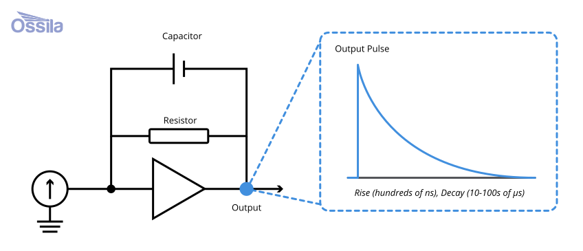
In these systems first, a photon or charged particle deposits energy in the detector, releasing a proportional amount of charge. Then a charge-sensitive preamplifier integrates that charge into a voltage step. Once this signal is collected, this information must be accurately processed to extract particle or photon energy.
Digital pulse processors contain a fast ADC directly after the preamplifier to continuously digitize the stepped waveform. This enables all further processing to happen with arithmetic operations on the sample stream, rather than running a signal through independent circuits (as with analog systems). Typical fast ADC sampling rates for spectroscopy-grade germanium and silicon systems range from 50 to 250 MS/s at 14 to 16 bits of resolution.

Digital architectures offer several structural advantages over their analog counterparts:
- As filters are defined by numerical algorithms rather than physical trim potentiometers and capacitors, component drift and age degradation will not affect these systems.
- You can directly set and record filter parameters, making experiments much more reproducible.
- You can fully inspect signal waveforms and intermediate filter stages, allowing for advanced system diagnosis.
However, digital conversion is not a guaranteed upgrade. Systems with an inferior ADC, an under sampled rise time, or a poorly optimized filter will not perform as well as a high-quality analog amplifier. The primary advantages of direct digitization are operational flexibility, environmental stability, and signal visibility, rather than artificial gains in fundamental resolution.
A digital pulse processor (DPP) is fundamentally two parallel filters analyzing a common sample stream, supported by event-management logic. This system contains many steps including a trigger channel, gated baseline tracking , trapezoidal shaping, pole-zero cancellation, pile-up rejection, signal discrimination and finally building the histogram. All of these are algorithmic functions that can be applied to the digital signal from the ADC.
Fast Trigger/ Timing Channel
This is a short filter, usually a fast differentiator acting as a narrow trapezoid or triangle, that responds in tens of nanoseconds. This fast pulse precisely marks an event’s arrival time and flags whether multiple events arrived simultaneously. The pulse is not used in energy measurement. Maintaining strict independence between this fast channel and the slower energy filter ensures neither process compromises the performance of the other.

Gated Baseline Tracking
Between events, the output must return to a known zero reference. Things like DC drift and the residual tails of previous pulses can introduce offsets, leading to incorrect measurement of the latter pulses. The system must continuously estimate and subtract a baseline to account for this. This is done by the gated-baseline tracking component.
Critically, this estimate must update only when the fast channel confirms no pulse is present. In other words, this correction must be a gated response.
Trapezoidal Shaping
This slow energy filter transforms each preamplifier step into a trapezoid whose flat-top height is proportional to the deposited energy. This specific filtering stage primarily dictates the ultimate energy resolution of the system.
Pole-zero Cancellation
The preamplifier step decays exponentially, and if left uncorrected, this decay causes the shaped pulse to subsequently undershoot. At high count rates, these offsets can accumulate and severely distort the energy spectrum.
Pole-zero cancellation mathematically removes this feature, ensuring the shaped pulse returns cleanly to the baseline. In a digital architecture, this is done using a numerical term in the filter mathematics tied directly to the preamplifier’s decay constant, rather than a manual hardware adjustment required for analogue systems.

Pile-up Rejection
When two events arrive closer together than the energy filter can resolve, their corresponding trapezoids overlap, making the combined amplitude meaningless. The fast channel flags this proximity and signals for both events to be discarded before the meaningless amplitude is recorded.

Because a fast-slow processor can only reject a pair if both events successfully fire the fast channel, the fast threshold is typically set as close to the noise floor as practically possible. However, there is a lower limitation of this pile up rejection. If events are too close together to be separated by the fast channel, they will still pile up and sum.
Lower- and upper-level discriminators (LLD/ULD)
Digital thresholds establish the range of pulse heights admitted to the histogram. The lower threshold rejects low-level noise and the electronic pedestal, while the upper threshold rejects overflow events. Unlike analog voltage comparators, these are numerical comparisons, allowing them to be adjusted, logged and reproduced precisely.
Histogram
Every accepted event is placed into the appropriate channel which matches its measured height. This builds a histogram, event by event, that forms the final energy spectrum.

Analog Systems
For decades, this process was performed with a rack of NIM modules, which many labs still use today. Reviewing this legacy chain block-by-block is useful, as modern digital systems reproduce most of these functions mathematically, rather than in hardware.
Most analogue systems contain:
- Charge-sensitive preamplifier: This unit integrates charge onto a feedback capacitor. This generates a voltage step with a fast rise (nanoseconds to a few hundred nanoseconds) and a slow exponential decay. There are resistive-feedback and reset-type preamplifiers. Resistive-feedback preamplifiers have decay time constants that can range from tens of microseconds for scintillation detectors, to hundreds of microseconds for HPGe systems. Reset-type preamplifiers instead step up voltage on every incoming pulse, discharging abruptly upon saturation.
- Shaping (spectroscopy) amplifier: This component is the core of the analogue chain. It consists of a differentiator followed by several integrators, the classic CR-(RC)n network. This transforms the initial pulse from the preamplifier into a quasi-Gaussian pulse a few microseconds wide, simultaneously filtering high frequency noise and shortening the pulse duration to be processed by future elements.
- Discriminator and single-channel analyser (SCA): A discriminator fires a logic pulse when the signal crosses a defined threshold. The SCA only allows signals of a certain energy through, creating a threshold. These only fires when a pulse falls inside a specific energy window.
- Peak-sensing ADC: Captures the maximum height of the shaped pulse and converts it to a corresponding channel number.
- Multichannel Analyzer (MCA) memory: Adds to the channel count. After millions of events, the accumulated histogram represents the energy spectrum.
Issues with Analogue Systems
This analog chain worked well for decades and continues to work well in many labs. However, it possesses inherent architectural limitations.
Gain and shaping depend on physical components and trim potentiometers, which drift with temperature and age. Two structurally identical amplifiers rarely produce identical spectra, and historical instrument settings rely entirely on manual logbook entries.
Furthermore, at high count rates, an AC-coupled baseline shifts, moving and broadening peaks. Large detectors also suffer from ballistic deficit which can be accounted for in digital pulse systems.
Finally, while the external amplifier output can be scoped, the intermediate stages inside the physical shaping network remain unobservable.
Why Use a Trapezoid Shaping Filter?
The trapezoidal shape is mathematically a near-optimal filter to use in environments where the two dominant electronic noise types are present, which is the case in these spectroscopy systems.
Electronic noise in these systems divides into two categories, which scale oppositely with shaping time.
- Series (voltage) noise is dominated by the input transistor. This increases with shorter shaping times and is suppressed by averaging over a longer interval.
- Parallel (current) noise which arises from detector leakage and similar sources. It increases with longer shaping times, as the system integrates more of this noise over time.
Combining both contributions, and introducing a roughly flat 1/f noise contribution, results in a characteristic U-shaped Noise-vs-Shaping Time curve. Initially, total noise falls as shaping time increases. This reaches a minimum where series and parallel contributions are roughly equal and then rises again. This minimum represents the optimal shaping time for a particular detector.
In order to counteract both series and parallel noise, the signal is shaped with an algorithm using certain parameters, including shaping time and peaking time. A trapezoidal recursive shaper algorithm provides the best approach to account for both noise sources. The rising and falling ramps of the trapezoid perform the necessary noise averaging. Extending the peaking time increases this averaging effect and improves resolution, up to the detector’s specific noise minimum.
The flat-top addresses a separate issue: ballistic deficit. In a large-volume detector, charge collection time varies depending on the physical location of the interaction within the bulk volume. For example, a large coaxial germanium detector may exhibit charge-collection times spanning several hundred nanoseconds. If the filter peaks and immediately falls, delayed charge pulses are measured inaccurately low, resulting in broadened spectral peaks. A flat top programmed to exceed the maximum charge-collection time effectively holds the measurement window open until essentially all charge has been integrated.
Longer shaping times yield better resolution but reduce overall system throughput. This creates an engineering trade off. Each event occupies the energy filter for roughly twice the peaking time plus the flat-top duration. This lowers the maximum event rate before pile-up dominates. Every incremental gain in resolution inherently increases system dead time.
The Recursive Trapezoidal Algorithm
The trapezoidal algorithm became the foundational standard of digital spectroscopy following two 1994 papers by Jordanov and Knoll. This work demonstrated that a trapezoidal or triangular shape can be built recursively (by reusing previous results rather than recomputing a full convolution at every sample). This way the algorithm executes in real time on efficient hardware architectures.
At each sample interval n, the filter processes a double delay-and-subtract signal followed by two running accumulations:
d[n] = v[n] - v[n-k] - v [n-l] + v[n-k-l-p]
p[n] = p[n-1] + d[n]
s[n] = s[n-1] + p[n] + M*d[n]
Here, v[n] is the input sample, the integer delay lengths k and l set the rise time (k samples) and the flat-top width (l-k samples). M is a decay-deconvolution constant tied to the preamplifier time constant τ of order:

where Tc is sthe sampling clock period. This functions as the digital pole-zero term. Setting the flat-top duration to zero degenerates the trapezoid into a triangle.
The primary engineering implication of this algebraic structure is that the entire filter, including pole-zero cancellation, is completely defined by a handful of integers and a single decay constant. Consequently, these parameters are precisely recordable and universally reproducible.
Viewing Status of DPP Components
An advantage of digital pulse processing is that you can observe intermediate stages during processing. In analog systems, each stage is a physical circuit so investigating each stage would require probing with an oscilloscope. In digital pulse processing, you can just observe their output on the system software.
Monitoring four primary diagnostic traces provides an overview of system performance:
| Trace | Diagnosis |
|---|---|
| Raw preamplifier trace | Confirms the decay time constant, reveals environmental noise or microphonics, and verifies whether the ADC’s dynamic range is being used optimally. |
| Fast-trigger output | Verifies that the discrimination threshold is cleanly above the baseline noise. |
| Trapezoidal energy filter | Should show a uniform flat-top that returns squarely to baseline.
|
| Baseline Estimate | Must remain steady and near zero. A baseline that wanders as a function of count rate indicates that the gating logic or restorer parameters need adjustment. |
Troubleshooting DPP Systems
Below are some tips for troubleshooting issues with your MCA or digital pulse processor.
Resolution worse than spec at low rate
The peaking time is likely too short. Lengthen it toward the noise optimum. If lengthening degrades resolution further, the optimum has been passed (parallel/leakage noise is dominating); shorten the peaking time instead.
Peaks broaden as count rate rises
Indicates pile-up and baseline effects. Shorten the peaking time to trade some resolution for throughput, and confirm that pile-up rejection is active.
Peaks shift position with count rate
A classic pole-zero or baseline-restoration error. Re-check the decay constant and the gated baseline settings. Centroid drift with rate is the tell-tale sign of baseline degradation.
Low-energy tailing on peaks
Often caused by genuine charge trapping in the detector, but incomplete baseline restoration and pole-zero error contribute. Check both settings before attributing the issue to the crystal.
High-energy tailing
The baseline not recovering before the next pulse arrives at high rates. Shorten the shaping time or improve pile-up rejection parameters.
Throughput too low / dead time too high
The trapezoid is too long for the current count rate. Reduce the peaking time and/or flat-top duration, accepting the associated resolution cost.
Spike of counts at the bottom of the spectrum
Indicates noise triggering. Raise the lower-level discriminator (LLD) and the fast-channel threshold.
Trapezoid flat-top tilting
Improper pole-zero cancellation (PZC). If the flat-top tilts upward, decrease the PZC decay constant (M or τ). If the flat-top droops downward, increase the PZC decay constant.
Trapezoid peak rounding or amplitude loss
Indicates ballistic deficit. Extend the flat-top duration and delay the peak sampling time to ensure full charge collection.
Explore More Resources
 Pole-Zero Cancellation
Pole-zero cancellation is an important part of radiation spectroscopy analysis. Converting charges created from radiation events, such as gamma rays produced in gamma spectroscopy, into binnable signals introduces a shaping error which can impact later analysis.
Read more...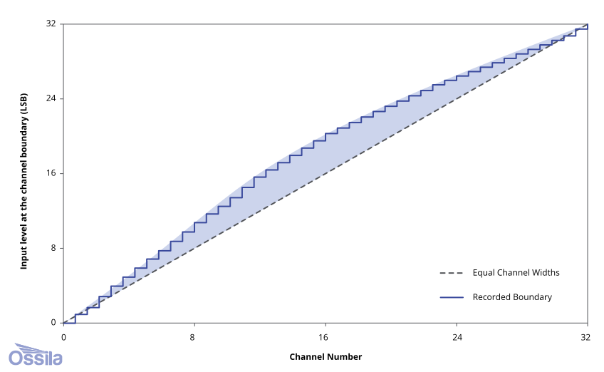 ADC Differential and Integral Non-Linearity
Differential nonlinearity and integral nonlinearity are the two specifications that determine whether an analogue-to-digital converter (ADC) is suited to pulse height spectroscopy. Both usually appear on an ADC’s datasheet.
Read more...Contributors
Written by
Product Developer
Diagrams by
Graphic Designer
References
- Multichannel Pulse Analysis, Radiation Detection and Measurement, G. F. Knoll, Wiley (2010)
- Digital synthesis of pulse shapes in real time..., G. F. Knoll, Nucl. Instr. Meth. A (1994)
- Digital techniques for real-time pulse shaping in radiation..., V. T. Jordanov, G. F. Knoll, A. C. Huber and J. A. Pantazis, Nucl. Instr. Meth. A (1994)
- Evaluation of real-time digital pulse shapers with various..., N. Menaa et al., Nucl. Instr. Meth. A (2011)