


ADC Differential and Integral Non-Linearity
Channel Widths in ADC | Differential Non-Linearity | Integral Non-Linearity | Number of Channels
Electronic Noise as Peak Width | Gain and Offset Drift | Linearity of a Full Instrument
Differential nonlinearity and integral nonlinearity are the two specifications that determine whether an analogue-to-digital converter (ADC) is suited to pulse height spectroscopy. Both usually appear on an ADC’s datasheet.
- Differential nonlinearity (DNL) describes how equal the channel widths are. This governs whether a smooth spectrum will appear smooth after processing.
- Integral nonlinearity (INL) describes how far the channel boundaries have wandered from a straight line. This determines whether channel number converts correctly into energy.
Another specification often quoted before INL or DNL for ADCs is bit depth or resolution. However, this has little bearing on non-linearity, and neither resolution or non-linearity alone describes how an assembled instrument will behave.
Channel Widths In ADC
A pulse height spectrum is a histogram. What distinguishes it from a histogram built in software is that its bin edges are set by comparator thresholds inside the ADC. Because these thresholds depend on the physical properties of the underlying components, they are never perfectly evenly spaced. INL and DNL are simply different ways of describing this unevenness.
A standard test makes the consequences easy to visualize. Each channel should cover an equal percentage of the ADC's input range. If a converter is presented with many pulses whose heights are spread evenly across its input range, every channel should collect the exact same number of counts. Therefore, a perfectly flat histogram is the pass condition, and any departure from it maps the converter’s imperfections.

Differential Nonlinearity
Suppose one channel happens to be 3% wider than it ought to be. Pulses will land in it 3% more often than in its neighbours, so it reads 3% artificially high. This is differential nonlinearity. The width error of an individual channel appears as a count error of the same size.

Missing Codes
This extreme case is the defect spectroscopists worry about most. A channel squeezed to zero width can never be landed in, so it records nothing regardless of the source or the counting time. This is a missing code. The counts it should have collected still arrive, landing in neighboring channels instead. The total count is preserved, but the shape is distorted.
Integral Nonlinearity
Uneven widths also have a second consequence unrelated to counts. Each channel boundary sits wherever the widths beneath it happen to add up to. For example, a group of channels running slightly wide near the bottom of the range pushes every boundary above them upwards. The displacement grows as more errors accumulate. Integral nonlinearity is that accumulated displacement, which appears as a curved energy calibration.
Ultimately, all three metrics come out of one measurement. When read one channel at a time, the width errors represent differential nonlinearity. Added up from the bottom of the range, they represent integral nonlinearity. If the width errors are extreme, the converter exhibits missing codes. They cause different types of damage, distorting the spectrum shape locally and bending the energy axis globally.
Differential Nonlinearity & Distortions
Unequal channel widths turn a smooth continuum into a structured one. As Knoll warns, the resulting artificial features can be easily misinterpreted as true physical structure in the spectrum, and nothing beyond the count effect described above is needed to cause this.
The resulting pattern is rarely random. Specific converter architectures produce distinct, predictable error signatures.
- Sub-ranging and pipeline converters carry their largest width errors at the boundaries between their internal ranges, which recur at regular intervals. For example, a 14-bit converter built from 5-bit stages has 32 of these boundaries, evenly spaced. Against an evenly spread input, the count deviation at these points reaches about 5% of the average channel content.
- Successive-approximation converters, including those in microcontrollers, exhibit similar structured errors at their major carry transitions. At these transitions, capacitor mismatch shifts the steps at the half and quarter marks of full scale.
Seeing any of this takes patience. Counting statistics give about 1% scatter in a channel holding ten thousand counts, meaning a 1% width error only matches the baseline noise. Measuring it properly requires several times more data. In other words, across 1024 channels, you would need tens of millions of events to see differential non-linearity. This is exactly why this measurement relies on a pulser rather than a physical source.
The classical remedy is the sliding scale, introduced in 1963. A known random offset is added to each pulse before conversion and subtracted afterwards, ensuring that one input amplitude samples many channel boundaries rather than always hitting the same one. Uniformity improves roughly with the square root of the number of channels the offset spans.
However, there are implications to reducing the offset span. The usable range shrinks by the span of the offset and channel profiles broaden. Also, mismatched add-and-subtract steps write a periodic pattern into the integral nonlinearity instead of removing it. As well as this, the systematic width errors do not average down.


Integral Non-Linearity & Energy Calibration
Integral nonlinearity determines whether channel number corresponds to energy in a true straight line. A standard two-point calibration establishes a zero point and a keV-per-channel slope. Any accumulated displacement left over appears as an energy error scaled by that keV per channel. Consequently, the same underlying defect will lead to a higher energy error in a system with a coarser energy axis.
Analyzers typically quote INL as a fraction of full scale. Some manufacturers specify below ±0.025% over the top 99.5% of the spectrum, while others report ±0.02% for a 16-bit unit using sliding-scale linearization. For context, Knoll’s guidance suggests systems should stay below 0.1% for INL, and a few percent for differential nonlinearity.
However, the practical significance of these numbers depends entirely on the detector. On a 2 MeV axis, a ±0.025% error translates to ±0.5 keV. For a germanium detector with a 1.8 keV resolution, that error consumes 28% of the resolution and significantly impacts centroid work. Conversely, that same ±0.5 keV is only about 1% of a NaI(Tl) scintillator’s peak width at 662 keV, meaning it can be safely ignored.
This sensitivity is why high-resolution germanium spectroscopy routinely incorporates a quadratic calibration term. In one large germanium array, actively correcting for converter nonlinearity narrowed the spread of calibration residuals from 0.1 keV to just 0.04 keV. Left uncorrected, the INL shifted a 1592.5 keV double-escape peak down by 0.45 keV and artificially widened it from 2.16 to 2.41 keV.
Finally, a brief note on interpreting published specifications. INL can be calculated using either endpoint-referenced or best-fit-referenced methods, which yield mathematically different results for the same converter. Additionally, because integrated converters inherently deviate near the extremes of their range, specifications often focus on the most linear region (such as the top 99.5%) to reflect standard operating conditions.

ADC Bit Resolution
Splitting the range into more channels does not change how evenly the boundaries are spaced. This is because boundary spacing is defined by components inside the converter. It simply divides the same counts among more bins.
If anything, more bits make achieving high uniformity harder. Component mismatch produces a roughly fixed error in volts, while each added bit reduces a channel’s width, so the same mismatch becomes a relatively larger error. Hence high resolution detectors rely on trimming, dither, and correction. Also, finer channels do not recover lost information. Rebinning a Gaussian peak conserves its fitted area to better than 0.01%, so extra channels do not improve a measurement of how many counts a peak contains.
What they do improve is shape fidelity, up to a point. Reliable peak fitting requires approximately 10 channels across a peak’s Full Width at Half Maximum (FWHM). Below 3 channels, the fitted width artificially inflates by a few percent. Beyond 10, extra channels only spread the same counts more thinly.
Detector resolution decides the useful number of channels. A NaI(Tl) scintillator yields roughly 7% resolution at 662 keV, about 46 keV wide. On a 2 MeV axis with 1024 channels, each channel is 1.95 keV. This puts 24 channels across that 662 keV peak, and 9 across a narrower peak at 100 keV. Germanium detectors at 1.8 keV resolution require about 0.25 keV per channel, demanding roughly 8192 channels total.
The native hardware resolution of modern converters far exceeds the necessary channel count for most detectors. Consequently, high-resolution continuous data is routinely binned down before histogramming. In advanced digital pulse processing instruments, this final channel count is treated as a highly flexible software setting, distinctly separate from the converter’s inherent hardware resolution.

Electronic Noise as Peak Width
Because detector resolution is traditionally quoted in keV at full width half maximum (FWHM), the electronics’ noise contribution must be evaluated in those same units rather than in decibels. For a typical Gaussian peak, this FWHM value is about 2.35 times the standard deviation.
Independent broadening mechanisms do not add to the noise linearly. Rather, they combine in quadrature:

The detector term accounts for statistical charge generation and collection effects, while the electronics term encompasses all downstream noise. By injecting a stable test signal, a pulser peak’s width can isolate and directly measure this electronics contribution.
Adding in quadrature inherently minimizes the impact of smaller noise sources. For instance, if the electronics contribute one-third of the detector’s native width, the overall resolution degrades by only 5%. Even an electronic contribution equal to the detector’s width only increases the total FWHM by 41%.
Quantization noise itself represents a relatively minor factor. Rounding a continuous pulse amplitude into a discrete channel distributes an error across that channel, equivalent to about 0.68 channels of peak width. A peak spanning 6 channels is consequently broadened by 0.6%, while one spanning 3 channels broadens by 2.5%. This coarse-binning bias can often be calculated and subtracted rather than simply tolerated.
In contrast, standard audio-centric ADC metrics, like signal-to-noise ratio (SNR), total harmonic distortion (THD), SINAD, and effective number of bits (ENOB), address a fundamentally different use case. These figures measure how faithfully a converter reproduces a single, large, continuous sine wave. IEEE Standard 1241 explicitly acknowledges this split, reserving SINAD and THD for waveform applications, while mandating DNL, INL, gain, and offset metrics for strict data acquisition. For example, a single missing code barely registers in a sine-wave distortion figure, yet it creates a permanent, catastrophic zero-count gap in a spectroscopic histogram.
Gain and offset drift between calibrations
While nonlinearity is a fixed characteristic of the converter’s hardware, gain and offset drift shift the entire energy axis over time between calibrations. In most measurement systems, the converter itself is rarely the dominant source of this drift.
For example, measured front-end gain drift in high-resolution germanium systems typically runs on the order of 100 ppm per hour (approximately 0.1 keV per hour at 1332 keV). In contrast, a high-quality converter’s gain coefficient contributes well under 0.01 keV per degree Celsius.
In scintillator-based systems, drift is almost entirely dominated by the detector itself. Published stabilization techniques have demonstrated the ability to reduce a cobalt-57 peak’s relative shift from roughly 19% down to 1%. Consequently, an ADC’s thermal specification remains a secondary operational concern until the detector’s inherent environmental instability is adequately managed.
Linearity of a Full Instrument
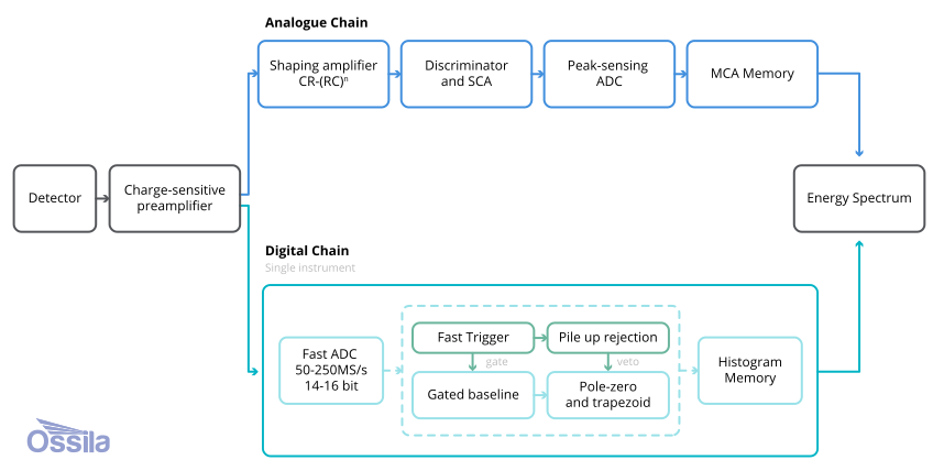
The ADC is ultimately just one element in a comprehensive capture chain that includes the preamplifier, shaping stage, baseline restoration, and peak detection. True instrument-level nonlinearity is dictated by the combined performance of this entire signal path.
One example of how different elements can affect linearity is to consider high count rates. As the event rate rises, differential nonlinearity artifacts can worsen because incoming pulses sit on the decaying tails of preceding events. Consequently, the actual amplitude reaching the converter depends heavily on signal history, which is a dynamic system behavior that standard component datasheets inherently cannot capture.
System architecture also plays a defining role in how these errors manifest. In a classical peak-sensing analyzer, the converter digitizes the peak amplitude exactly once, causing its inherent channel width errors to map almost directly onto the final spectrum channels.
In contrast, modern digital pulse processing instruments use a free-running converter where the final spectrum channel is the result of advanced digital signal processing, such as trapezoidal filtering. Because the digital filter evaluates and averages over many continuous samples, individual ADC width errors are largely dithered away. However, it is worth noting that severe structured errors at internal range boundaries may still survive the filtering process.
Learn More
 Digital Pulse Processors
In pulse-mode radiation spectroscopy, each electrical pulse carries information about the energy deposited by the quantum of radiation that produced it, proportional to its amplitude.
Read more...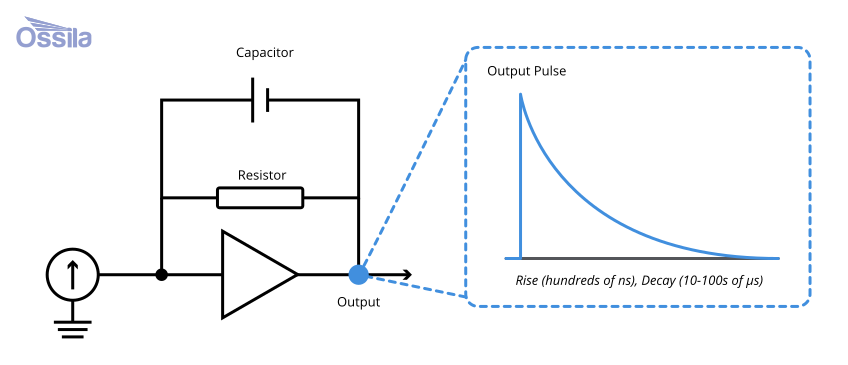 Pole-Zero Cancellation
Pole-zero cancellation is an important part of radiation spectroscopy analysis. Converting charges created from radiation events, such as gamma rays produced in gamma spectroscopy, into binnable signals introduces a shaping error which can impact later analysis.
Read more...Contributors
Written by
Product Developer
Diagrams by
Graphic Designer
References
- A New Method for Analog to Digital Conversion, C. Cottini, E. Gatti, V. Svelto, Nucl. Instr. Meth. A (1963)
- ADC Nonlinearity Correction for the Majorana Demonstrator, N. Abgrall, J. M. Allmond, I. J. Arnquist, et al., IEEE Trans. Nucl. Sci. (2021)
- Radiation Detection and Measurement (Multichannel Pulse Analysis), G.F. Knoll, Wiley (2010)
- Digital Synthesis of Pulse Shapes in Real Time..., V. T. Jordanov and G. F. Knoll, Nucl. Instr. Meth. A (1994)
- Practical Gamma-ray Spectrometry, G. Gilmore, Wiley (2008)