Calculate Sheet Resistance Using the Four-Probe Method
Sheet resistance (also known as surface resistance or surface resistivity) is a common electrical property used to characterize thin films of conducting and semiconducting materials. It is a measure of the lateral resistance through a thin square of material, i.e. the resistance between opposite sides of a square. The key advantage of sheet resistance over other resistance measurements is that it is independent of the size of the square—enabling an easy comparison between different samples.
This property can easily be measured using a four-point probe and is critical in the creation of high-efficiency perovskite photovoltaic devices, where low sheet resistance materials are needed to extract charge.
Four-Point Probe

Applications of Sheet Resistance
Sheet resistance is a critical property for any thin film of material in which electrical charges are intended to travel along (rather than pass through). For example, thin-film devices (such as perovskite solar cells or organic LEDs) require conducting electrodes which generally have thicknesses in the nanometer to micrometer range. The figure below shows how charges move within an LED device. The electrodes must transport electrical charge laterally and need low sheet resistances to reduce losses during this process. This becomes even more important when attempting to scale up the size of these devices, as the electrical charges will have to travel further along the electrodes before they can be extracted.

Furthermore, the resistivity and conductivity can be calculated if the sheet resistance and material thickness are known. This allows for the materials to be electrically characterized, purely by taking a sheet resistance measurement.
The Four-Probe Method for Measuring Sheet Resistance
General Theory
The primary technique for measuring sheet resistance is the four-probe method (also known as the Kelvin technique), which is performed using a four-point probe. A four-point probe consists of four equally spaced, co-linear electrical probes, as shown in the schematic below.

It operates by applying a DC current (I) between the outer two probes and measuring the resultant voltage drop between the inner two probes.
The Sheet Resistance Equation
The sheet resistance can then be calculated using the following equation:

Rs is the sheet resistance, ΔV is the change in voltage measured between the inner probes, and I is the current applied between the outer probes. The sheet resistance is generally measured using the units Ω/□ (ohms per square), to differentiate it from bulk resistance.
It should be noted that this equation is only valid if:
- The material being tested is no thicker than 40% of the spacing between the probes
- The lateral size of the sample is sufficiently large
If this is not the case, then geometric correction factors are needed to account for the size, shape, and thickness of the sample. The value of this factor is dependent on the geometry being used.
If the thickness of the measured material is known, then the sheet resistance can be used to calculate its resistivity:

Here, ρ is the resistivity, and t is the thickness of the material.
Eliminating Contact Resistance
One of the primary advantages of using a four-point probe to perform electrical characterization is the elimination of contact and wire resistances from the measurement. The diagram below shows the circuit resistances of a four-point probe measurement..

The applied current I enters and leaves the sample via the outer probes, and flows through the sample. Voltmeters typically have high electrical impedance to prevent them affecting the circuit being measured, so no current will flow through the inner two probes. Only the voltage is measured between the inner probes, meaning that the wire resistances (RW2 and RW3) and the contact resistances (RC2 and RC3) do not contribute to the measurement. Any measured decrease in voltage (ΔV) will therefore arise entirely from the sample resistance (RS2). This simplifies the sheet resistance equation, so that only ΔV and the applied current are required to find the value of RS2 (i.e. the sheet resistance).
Geometric Correction Factors
Whilst the above equation for sheet resistance is independent of sample geometry, this only applies when the sample is significantly larger (typically having dimensions 40 times greater) than the spacing of the probes, and if the sample is thinner than 40% of the probe spacing. If this is not the case, the possible current paths between the probes are limited by the proximity to the edges of the sample, resulting in an overestimation of the sheet resistance. To account for this difference, a correction factor based upon the geometry of the sample is required.
All the correction factors in this guide were obtained from Haldor Topsøe, Geometric Factors in Four Point Resistivity Measurement, 1966.
Circular Samples
For a circular sample of diameter d, measured at the center of the sample, the correction factor can be calculated using:
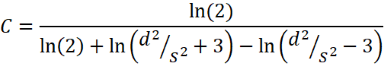
Where s is the distance between probes. For d >> s this equation tends to unity, enabling the use of the uncorrected equation.
Rectangular Samples
For a rectangular sample, the determination of the geometrical correction factor is slightly more complicated as there is no equation. Instead, a table of empirically-determined correction factors is used. The values in this table only apply when the probes make contact in the center of the sample, and are aligned parallel to the sample's longest edge (l), as shown below.

As an example, suppose the rectangular sample shown in the figure above has a long edge of l = 20 mm and short edge of w = 10 mm, and the spacing of the probes being used is s = 2 mm. In this case, l / w = 2 and w / s = 5, so the table is searched for the correction factor which satisfies these two values, looking along the columns for l / w = 2 and the rows for w / s = 5, which is C = 0.7887. The measured sheet resistance is multiplied by this value to get the correct value for the sample.
|
w / s |
l / w = 1 |
l / w = 2 |
l / w = 3 |
l / w = 4 |
|
1 |
|
|
0.2204 |
0.2205 |
|
1.25 |
|
|
0.2751 |
0.2751 |
|
1.5 |
|
0.3263 |
0.3286 |
0.3286 |
|
1.75 |
|
0.3794 |
0.3803 |
0.3803 |
|
2 |
|
0.4292 |
0.4297 |
0.4297 |
|
2.5 |
|
0.5192 |
0.5194 |
0.5194 |
|
3 |
0.5422 |
0.5957 |
0.5958 |
0.5958 |
|
4 |
0.6870 |
0.7115 |
0.7115 |
0.7115 |
|
5 |
0.7744 |
0.7887 |
0.7887 |
0.7887 |
|
7.5 |
0.8846 |
0.8905 |
0.8905 |
0.8905 |
|
10 |
0.9313 |
0.9345 |
0.9345 |
0.9345 |
|
15 |
0.9682 |
0.9696 |
0.9696 |
0.9696 |
|
20 |
0.9822 |
0.9830 |
0.9830 |
0.9830 |
|
40 |
0.9955 |
0.9957 |
0.9957 |
0.9957 |
| ∞ |
1 |
1 |
1 |
1 |
Not every sample will fall neatly into these categories. If this is the case, it is recommended that cubic spline interpolation is used to estimate the appropriate correction factor for the sample.
It is important to note that the correction factors for circular and rectangular samples detailed above only apply for measurements taken in the center of the sample. If the measurement is not in the center, different correction factors are needed.
Other Shapes and Probe Positions
For different sample shapes and for measurements not performed at the center of the sample, alternative correction factors are required. Most of these can be found in Haldor Topsøe, Geometric Factors in Four Point Resistivity Measurement , 1966, or F. M. Smits, Measurement of Sheet Resistivities with the Four-Point Probe , Bell Syst. Tech. J., May 1958, p. 711.
If the shape of the sample is irregular, consider whether it is closer to rectangular or circular and then estimate what size of that shape could fit within the sample.
Thick Samples
If the sample being tested is thicker than 40% of the probe spacing, an additional correction factor is required. The correction factor used is dependent upon the ratio of the sample thickness (t) to the probe spacing (s) and some of the possible values are listed in the table below:
|
t / s |
Correction Factor |
|
0.4 |
0.9995 |
|
0.5 |
0.9974 |
|
0.5555 |
0.9948 |
|
0.6250 |
0.9898 |
|
0.7143 |
0.9798 |
|
0.8333 |
0.9600 |
|
1.0 |
0.9214 |
|
1.1111 |
0.8907 |
|
1.25 |
0.8490 |
|
1.4286 |
0.7938 |
|
1.6666 |
0.7225 |
|
2.0 |
0.6336 |
As with the rectangular samples, if t / s does not equal one of the values given in the table, a cubic spline interpolation is recommended to estimate the appropriate correction factor for the sample.
Four-Point Probe Equation Derivation
In order to determine how the sheet resistance of a thin film is measured using a four-point probe, a simplified scenario must first be evaluated. Imagine an arbitrarily sharp probe contacting and injecting current (through an applied voltage) into a semi-infinite volume (infinite in all directions except towards the probe) of a conductive material.

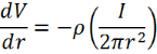
The current travels outwards from the point of contact through concentric hemispherical shells of equipotential, each of which have current density (J) of:

Where r is the radial distance from the probe (2πr2 being the surface area of the hemisphere). By applying Ohm’s Law (E = ρJ) with the electric field across each shell equal to the voltage drop over the shell thickness, or -ΔV / Δr (this term is negative as voltage decreases with r), and with the thickness of the shell tending towards zero, the following equation is obtained:
This can be integrated between r and r’ to obtain:

By applying the boundary condition that V approaches zero as r approaches infinity, the equation simplifies to:

Now imagine that there are four arbitrarily sharp probes (labeled 1 to 4) in contact with the semi-infinite conducting material, which are in a line with equal spacing (s). They are set up so that current is injected through probe 1 and collected by probe 4. If equivalent boundary conditions are assumed for each probe, the voltage at any point is equal to the sum of the voltage due to each probe separately, i.e.:
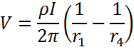
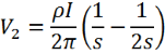
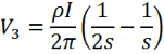
Where r1 and r4 are the radial distances from probe 1 and probe 4 respectively. Measurements of the voltage are then made between probes 2 and 3. Using the above equation, the voltage at probes 2 and 3 are:
Hence, the change in voltage (ΔV) between probes 2 and 3 is:
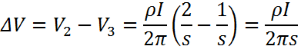
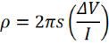
Therefore, the resistivity between the probes is:
This expression only applies in the case of a semi-infinite volume, and does not apply in the case of a thin film. However, a new expression can be derived using a similar analysis. As before, imagine the arbitrarily sharp probe contacting and injecting current into a thin film of material with thickness t.

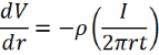
In this case, the current travels away from the probe (through the material) in short cylindrical shells of equipotential, each with a current density of:

By applying the same conditions for the electric field as previously (Ohm’s Law and shell thickness tending to zero), the electric field across each shell is:
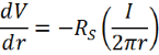
The resistivity has already been defined as the sheet resistance multiplied by the thickness of the materials, so this can be replaced in the above equation to give:
This can be integrated between r and r’ to obtain:
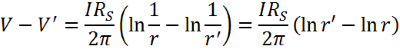
Unlike before, it cannot be assumed that the voltage tends to zero as r approaches infinity as the natural logarithm of infinity is not zero. However, this does not impact the analysis as the difference in voltage at different points (ΔV) is the value measured by the four-point probe.
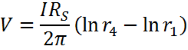
Now imagine the four-probe system in contact with a thin film, with an additional condition that the thickness of the film (t) is negligible compared to the probe spacing (s). For current being injected by probe 1 and collected by probe 4, the equation becomes:
The voltages measured at probes 2 and 3 are therefore:
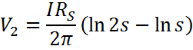
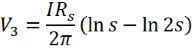
Hence, the change in voltage is:

Which can be rearranged to give:
Therefore, by measuring the change in voltage between the inner probes and the applied current between the outer probes, we can measure the sheet resistance of a sample.
Fast and Accurate Sheet Resistance Measurements
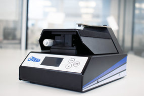

The Ossila Four-Point Probe makes the measurement of sheet resistance, resistivity, and conductivity of thin films quick and easy.
Four-Point Probe
Learn More
 Getting Started with the Ossila Four-Point Probe
The four-point probe is the most commonly-used piece of equipment for measuring the sheet resistance of a material.
Read more... How to Measure Sheet Resistance using a Four-Point Probe
This guide gives an overview of how to use the Ossila Four-Point Probe System, as well as some general tips and tricks for measuring sheet resistance.
Read more...References
- The 100th anniversary of the four-point probe technique: the role of probe geometries in isotropic and anisotropic systems, I. Miccoli et al., J. Phys.: Condens. Matter, 27, 223201 (2015)
- Resistivity Measurements on Germanium for Transistors, L. B. Valdes, Proceedings of the I.R.E, February, 420 (1954)
- Geometric Factors in Four Point Resistivity Measurement, H. Topsøe, (1966)