What is Voltammetry? Types and Applications

Jump to: Sweep Voltammetry | Polarography Methods | Pulse Voltammetry | Chronoamperometry
Differential Pulse Voltammetry | Additional Methods | Notes and Definitions
Voltammetry is a class of electrochemical techniques in which the current response of a solution is measured as a function of an applied potential. This encompasses a number of different methods for studying the kinetics and thermodynamics of electron gain (reduction) and electron loss (oxidation). In addition, voltammetry techniques can be used to test for the presence of an electroactive substance.
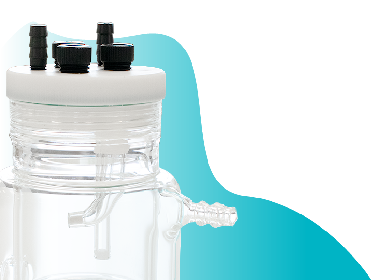
All voltammetric experiments share the same basic setup: an electrochemical cell containing three electrodes immersed in solution. The working electrode is where the reaction of interest takes place. The reference electrode provides a stable, known potential against which the working electrode potential is measured. The counter electrode completes the circuit, allowing current to flow without passing through the reference. A potentiostat controls the potential of the working electrode and measures the resulting current.
Different types of voltammetry vary in how the voltage is applied (it can be swept continuously, stepped in pulses, or oscillated) and the type of working electrode used. Each approach has different strengths and limitations in terms of sensitivity, output information, and the systems it is suited to.
Potentiostat
Sweep Methods
Cyclic Voltammetry
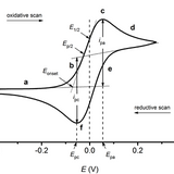
In cyclic voltammetry, potential difference is varied at a constant rate between two potentials. The direction of the voltage sweep reverses when the limiting potential is reached.

The main advantages of cyclic voltammetry over other voltametric methods are that it's easy to do and easy to analyze, as well as how large potential ranges can be examined rapidly. Cyclic voltammetry produces this signature "duck" current voltage curve, from which anodic and cathodic peak potential, onset potentials and other key metrics can be easily read. The reversibility of oxidation and reduction, and the approximate formal potential can be readily extracted from a compound’s cyclic voltammogram.

Cyclic voltammetry can be used to determine (or measure) a number of electrochemical properties about a material, including:
- The reversibility of a reaction
- The formal reduction potential of a species
- Electron transfer kinetics
- Energy levels of semiconducting polymers
Linear Sweep Voltammetry
Linear sweep voltammetry is one of the simplest voltammetry experiments, where only a single linear sweep is run. It is essentially measuring the forward half of a cyclic voltammetry sweep. This method is useful for studying irreversible reactions, where the reverse sweep would not provide more information.

Several key parameters can be observed from a linear sweep measurement. For example, linear sweep voltammetry can be used to determine thermodynamic reversibility based on:
- The peak current
- The peak current potential
- The half-peak current potential
Staircase Voltammetry
Staircase voltammetry is where the electrode is held at various potentials and the current is recorded after a set delay. The current is tracked over several "step changes" within the desired potential range. This applied potential waveform looks like a stair case. This is considered a multipotential pulse technique.

The method was designed for use with polarographic electrodes, but is today used with more standard electrodes. The results of this technique are similar to linear sweep voltammetry, and several staircases can be combined to create an analog for cyclic voltammetry. The purpose of this technique is to do cyclic voltammetry / linear sweep voltammetry while suppressing charging currents. This technique, however, has not found wide application. In order to reduce the charging currents sufficiently, the sampling rate and scan rate must be low, preventing fast scans. In addition, this method has poor signal to noise ratios.
Polarography Methods
Polarography is a very early form of voltammetry measurement, invented in 1922 by Jaroslav Heyrovský, for which he won the 1959 Nobel prize for chemistry. Initially the technique was developed for use with a dropping mercury electrode, but in the 1980s the static mercury electrode was developed to improve on the design. In addition, some methods have been modified to use more standard non-polarographic electrodes.
Polarographic electrodes are designed to form a mercury drop at a given potential. The mercury drop grows, until either the flow of mercury is stopped (static mercury electrode), or the drop falls off (dropping mercury electrode). For the static mercury electrode, the drop is often formed prior to changing the potential, and then knocked off after a result is recorded. In both cases, the fall of the mercury from the electrode effectively stirs the solution, largely reproducing the starting condition prior to the initial drop formation.
Polarographic methods are usually used in pulsed voltammetry techniques.
Conventional / DC Polarography1
The original form of polarography is referred to as DC polarography or conventional polarography. In conventional polarography the potential is varied slowly (1–3 mV s-1), such that each drop experiences a roughly constant potential. In modern practice, this method is often implemented with a small change in potential (1–10 mV) at the start of each drop instead. This technique can be used to measure the concentration of a known compound, calculate diffusion constants, find the polarographic half wave potential and calculate kinetic parameters in an irreversible system.
Pulse Voltammetry
Pulsed voltammetry encompasses several techniques in electrochemistry, but all require an electrode to be held at a potential for some time before progressing to another potential. This process may be repeated a number of times.
A key advantage of pulse voltammetry over sweep methods, such as cyclic voltammetry and linear sweep voltammetry, is the reduction of charging current effects and analyte depletion. In sweep methods, the electrode spends extended time at potentials where electrolysis occurs, gradually depleting the redox-active species near the electrode surface. Pulse voltammetry aims to address this by applying brief potential pulses and sampling the current towards the end of each pulse, where the charging current has decayed but the faradaic signal remains. Pulse voltammetry was originally designed for polarographic electrodes but can use any electrode.

In normal pulse voltammetry, the electrode is initially held at a voltage at which minimal electrolysis occurs. Subsequently the electrode is pulsed to a higher potential for a short period (1–100 ms), and the current is recorded at a point within that period, usually towards the end of the pulse.
It is important to have a gap between applying the potential and the current measurement. In the early time period, there is a charging current which decays with a time constant of RuCd, where Ru is the uncompensated resistance, and Cd is the differential capacitance of the double layer. RuCd is referred to as the cell constant and has value on the order of 10–1000 μs. By recording current after a time gap, the charging currents effects can be minimized.
However, even when charging currents are minimized, background currents can still impact a measurement. Background currents come from the non-ideal nature of the electrode, the electrolyte, or the purity of the system.
The key requirement here is that the diffusion layer is adequately renewed between pulses. With solid electrodes, this renewal relies on reversal of the redox reaction at the baseline potential, through natural diffusion or forced convection from a rotating electrode. Evidence for a lack of renewal of the diffusion layer would be appear as a distinct peak current (like in cyclic voltammetry) in the voltammogram, instead of asymptotically approaching a value.
Reverse Pulse Voltammetry1
The pulse scheme for reverse pulse voltammetry is very similar to normal pulse voltammetry. However, in reverse pulse voltammetry, the pulse aims to reduce potential of the system, whereas in normal pulse voltammetry, the pulse increases the potential experienced by an electrode. While in normal pulse voltammetry, the rest potential drives no electron transfer, in reverse pulse voltammetry, the initial set-up is designed such that current is at its maximum outside of pulse exposure.
Squarewave Pulse Voltammetry1
Squarewave voltammetry is a method which combines the sensitivity of pulse voltammetry, with the ability to test products directly as with cyclic voltammetry. However, it lacks the easy qualitative information of the prior methods.

This method starts at a potential and is pulsed negatively then positively by a potential (∆Ep ), before repeating a positive and negative pulse around a new potential which adds a step (Estep).
The current is usually recorded towards the end of each pulse, and the three different values plotted. These values are the forward current (where ∆Ep> is added), the reverse current (where ∆Ep is subtracted), and their difference is plotted. The pulse length tends to be 1 – 500 ms, the pulse height 50/n mV, and the step height 10/n mV.
Chronoamperometry
In the pulse voltammetry methods above, current is sampled at a single point after each pulse. Chronoamperometry instead records the full current-time transient following a potential step. This time-resolved response can be used to extract fundamental electrochemical parameters such as diffusion constants and electrode area.
Differential Pulse Voltammetry1
Differential pulse voltammetry offers increased sensitivity compared to normal pulse voltammetry. The differences between it and pulse voltammetry are:
- The base potential increases in small increments. This base potential serves to refresh the diffusion properties of the system.
- The pulse height is maintained at between 10-100 mV above the base potential
In addition, two currents are recorded, one before the pulse and one just before the end of the pulse. The difference (δi) between the two recorded currents is plotted verses the base potential. Normally the rest period is 0.5 - 4 s, and the pulse width is approximately 50 ms.

The results differ substantially from reverse pulse voltammetry and normal pulse voltammetry, and have a peak as opposed to a monotonic increase. The initial base potential can be interpreted as making a new apparent bulk concentration, different from what exists before. As the pulse height is decreased, the result tends towards the differential of the result of normal pulse voltammetry, giving a qualitative view of the results.
Additional Methods
Rotated Electrode Voltammetry1
Using rotating electrodes changes both the way compounds diffuse towards the working electrode and how the current is recorded. The main advantage of this method is that a steady state is quickly established with a high rate of mass transfer, increasing the limiting current. In addition, the rate of stirring can be controlled to affect the electronic processes. Steady state current measurements also have the advantage of reducing the impact of charging currents.
The main electrode used for these techniques is the rotated disk electrode. Rotated disk electrodes can be used for pulse voltammetry methods, or linear sweep methods.
Stripping Voltammetry1
In stripping voltammetry, the concentration of an electroactive species is increased at the electrode of interest, prior to analysis. This method allows for the study of electroactive species in highly dilute solution (10-10 – 10-11 M). The most common method of concentrating the electroactive species is to use an electrode that adsorbs or captures the electroactive species onto its surface. Alternatively, material can be deposited directly onto the electrode before analysis. The species is then "stripped" (i.e. redissolved) and analyzed, most commonly by linear sweep voltammetry or differential pulse voltammetry.
If the species is reduced prior to the method, and oxidized as it is released, it may be referred to as anodic stripping voltammetry. Alternatively, if it is oxidized before analysis and reduced during analysis, it is referred to as cathodic stripping voltammetry. Some species adsorbs on the electrode, without requiring electrolysis, and this is referred to as adsorptive stripping voltammetry.
Ultramicroelectrodes1
An ultramicroelectrode is characterized as having a smaller electrode area than the diffusion layer generated in the experiment. At very small electrode sizes, diffusion to the electrode becomes temporally independent, creating a steady state. This means that linear diffusion cannot be assumed.
Ultramicroelectrodes have the advantage of being able to operate within much shorter timescales than standard electrodes. This is because the standard electrodes take time to respond when the applied potential is changed. The potential of the electrode approaches the applied potential, via a decay with time constant of the "cell time constant". It takes approximately 5 cell time constants to reach the desired potential. This cell time constant reduces with electrode size. Faster scan rates are also possible in cyclic voltammetry using ultramicroelectrodes.
A further advantage of ultramicroelectrodes is that they substantially reduce the impact of iR drop. Because ultramicroelectrodes are so small, they generate smaller currents than conventional electrodes — typically in the pA to nA range. Since ohmic error is directly proportional to the current flowing (ΔE = i × Ru), this means that even in solutions with high uncompensated resistance, the potential error at the electrode surface remains negligible. This makes ultramicroelectrodes particularly well-suited to measurements in non-aqueous solvents, ionic liquids, or other poorly conducting media where conventional electrodes would produce unacceptably large iR errors.
Electrochemical Impedance Spectroscopy1
In electrochemical impedance spectroscopy, an oscillating AC voltage is applied to the electrochemical cell at a range of frequencies. This is applied alongside a fixed DC bias. Properties like solution resistance, charge transfer and diffusion can change depending on the AC frequency.
These small amplitude oscillations are repeated many times at each frequency, generating many repeated measurements. This increases EIS precision (compared to linear voltammetry) as you can average results over periods of time, increasing signal to noise ratio.
In addition, diffusion in EIS is usually simplified, and the range of frequencies which can be studied is large. What is measured is the impedance (i.e. the effective resistance and capacitance at the frequency used) of the cell at various frequencies.
This method outputs "faradaic impedance" i.e. the impedance from the oxidation and reduction at the electrode surface. The faradaic impedance must be separated from the impedance corresponding to the solution resistance, and the electrode charging. As with other voltammetry techniques, the faradaic impedance can be obtained by subtracting the impedance measured with no electroactive species present. However, the faradaic impedance can also be found by fitting the impedance spectrum to an equivalent circuit model.
Alternating Current Polarography1
An AC current can be combined with a pulsed voltage like those used in pulse voltametric methods. In such a method, the alternating current occurs at a much faster rate (usually oscillating at the rate 101–105 Hz) than the pulse, and to a much lower magnitude. Between pulses, the diffusion layer is renewed, either stirring or by a mercury drop dropping. The method works by the pulse setting up the ratio of oxidized and reduced compounds desired, and the AC pulse measuring them. As such, it is common to set up the system with only one of the oxidized or reduced forms.

Alternating Current Voltammetry1
An alternating current (AC) pulse can also be combined with linear sweep(s) to create alternating current voltammetry. The AC pulse must be much faster than the sweep rate for this technique and is usually in the range 101–105 Hz. Similar to alternating current polarography, the aim of the sweeping potential is to change the concentration of compounds local to the electrode.
The maths of this system is largely very similar to alternating current polarography, and hence its applications are also similar. In fact, if the electrochemical process is reversible at the scan rate of the linear sweep, all of the applications listed in the alternating current polarography section apply.
Notes and Definitions
Linear diffusion1
Most electrodes can be approximated as having linear diffusion on short time scales. The larger the electrode, and the shorter the time observed, the more the linear diffusion approximation applies. For example, for a 0.1 cm spherical electrode with reasonable diffusion terms, the linear treatment holds within 10% for 3 s. The equations on this page assume linear diffusion.
Cell time constant1
In electrochemical experiments, the electrodes take some time to reach an applied potential. The charging of the electrode produces a so-called charging current, which decays on the time scale of the "cell time constant". This puts a limit on how much time must be left after a potential change before recording a current. In addition, when potential is scanned, there is a maximum scan rate which can be applied due to the cell time constant. Essentially, the cell time constant means that after a potential pulse, current cannot be recorded on time scales shorter than a millisecond for standard electrodes. Ultramicroelectrodes allow recording on shorter timescales than milliseconds.
Potentiostat
Learn More
 Cyclic Voltammetry Basic Principles, Theory and Setup
Cyclic voltammetry is an electrochemical technique used to measure the current response of a redox active solution to a linearly cycled potential sweep.
Read more...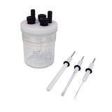 Linear Sweep Voltammetry: Introduction and Applications
Linear sweep voltammetry (LSV) is a simple electrochemical technique. The method is similar to cyclic voltammetry.
Read more...Related Products
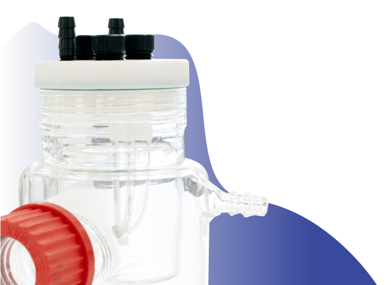
Photoelectrochemical Cells
Explore our range in photoelectrochemical cells.
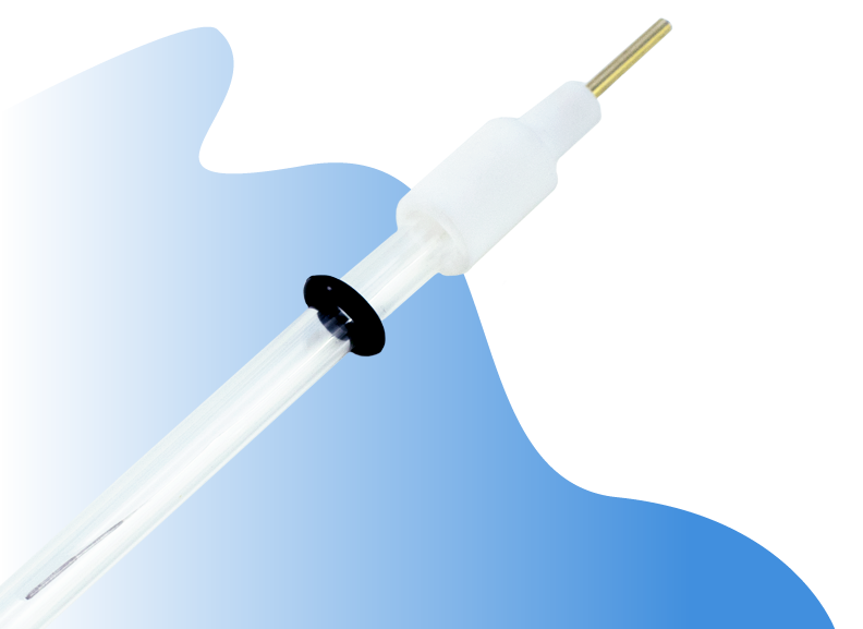
Electrodes
Explore our range of electrodes, including the glassy carbon working electrode.
References
- A. J. Bard and L. Faulkner, Electrochemical Methods: Fundamentals and Applications, John Wiley & son, 2nd edn., 2001.
- J. Heinze, Angew. Chemie Int. Ed. English, 1984, 23, 831–918.
- G. A. Mabbott, J. Chem. Educ., 1983, 60, 697.