It looks like you are using an unsupported browser. You can still place orders by emailing us on info@ossila.com, but you may experience issues browsing our website. Please consider upgrading to a modern browser for better security and an improved browsing experience.
Fluorescence spectroscopy measures fluorescence, a process where light is quickly reemitted from a material absorbing incident photons. Unlike phosphorescence, fluorescence occurs almost instantly, making it ideal for analyzing optical properties in materials. Fluorescence spectroscopy can be used to measure a broad range of samples including organic materials, semiconductor devices, optoelectronic materials and biological samples. The term fluorescence is often used interchangeably with photoluminescence.
Using a high energy light source, such as a UV light or a laser, a sample is stimulated with a specific wavelength to excite electrons into to a higher energy state. As the excited electrons return to ground state, the intensity of emitted light is measured across various wavelengths. This creates a fluorescence spectrum for a material, revealing key emission peaks.
Simply put, fluorescence occurs when an electron in an excited electronic state of a molecule, usually S1, quickly relaxes to the ground state S0, emitting a photon. These electronic states, their accompanying vibrational states (v1, v2, v3) and the transitions between them can be represented using Jablonski diagrams.
Jablonski diagrams showing the energy transitions involved in fluorescence
These are the main stages involved in fluorescence:
Absorption
The molecule absorbs light energy, exciting an electron from its ground state into a higher electronic state, for example from S0 to S1. The electronic level (and the subsequent vibrational level) the electron enters depends on the energy of the incoming photon.
Vibrational Relaxation
The excited electron loses some vibrational energy through non-radiative routes. This occurs until the electron reaches the lowest vibrational level of the electronic state, e.g. from S1v2 → S1v0).
Fluorescence
The electron returns to the ground state (S1 → S0), emitting a photon in the process.
Vibrational Relaxation Part 2
Another thing to note is the during fluorescence, the electron could relax into one of the vibrational states of the ground state (i.e. S0v1). It will then lose this energy via further vibrational relaxation.
In fluorescence spectroscopy, the electron becomes excited by absorbing a photon. However, fluorescence measurements are also useful for studying the materials used in electroluminescent devices like OLEDs. Often when people talk about fluorescence, they are referring mainly to the step 3 transition.
Key Fluorescence Characteristics
One of the main characteristics that defines fluorescence is the very short time between photon absorption and emission (usually ~10 nanoseconds). This differentiates it from phosphorescent materials which have much longer fluorescence lifetimes.
Some of the main properties that define fluorescence are the emission spectrum and intensity, fluorescence lifetime and quantum yield.
Emission Spectrum, Peak Wavelengths & Intensities
The energy of the photon emitted during fluorescence will be equal to the energy gap between the two transition states. The energy of this photon will correspond to its wavelength via the following equation:
By noting the wavelength of emission peaks in a spectrum, you can probe the energy transitions of a material, learning more about its molecular structure. Additionally, by measuring the intensity of emission at certain peaks, the rate or extent of a reaction or binding event can be determined. This is an especially useful non-invasive method for studying biological processes.
Fluorescence Lifetime
Fluorescence lifetime represents how long an excited electron can remain in its excited state before returning to S0. This is important to know as it affects the potential applications of the fluorophore (i.e. will it be suitable for LEDs, PV, biological markers, etc?). This also tells you how much time the excited fluorophore will have to react with its environment.
Fluorescence lifetime is influenced by three main factors: the average time needed for fluorescence to occur, known as the emissive rate (Γ); the rate of non-radiative decay processes (knr); and the rate of energy transfer (kt). All three contribute to determining how long a fluorophore remains in the excited state before returning to the ground state.
Quantum Yield
Simply put, quantum yield (or Photoluminescent Quantum Yield) is the ratio of the number of photons that enter the system compared to the number of photons you get out. This is important as the higher the quantum yield, the brighter the emission of your fluorophore.
As well as calculating these values, you can determine quantum yield and fluorescence empirically. Yield you can estimate by integrating the areas underneath the emission and absorbance spectrum and taking the ratio of these values.
Example quantum yield empirical measurement: The spectra without (dark blue) and with (light blue) the sample in place. The PLQE of the sample is given by integrating the emission area (light blue shaded area on the right) divided by the light absorbed area (dark blue shaded area on the left) (x100).
Rules of Fluorescence Spectroscopy
Here, we discuss some general rules which can be useful to bear in mind when doing fluorescence spectroscopy. These are not hard and fast rules – they are often broken. However, you may see these phenomena pop up again and again.
Mirror Image Rule
The mirror image rule states that often the absorbance spectrum of a fluorescent material is the mirror image of its emission spectrum.
Mirror image rule
In short, this happens due to the vibrational energy states in a material. During absorbance, an electron can be excited into a higher vibrational energy state. For example in the above Jablonski diagram, an electron can be excited into S1v0, S1,v1 or S1,v2, leading to peaks at three different wavelengths in the absorbance spectrum. Any electrons excited into a higher energy state will lose this energy through processes like thermalization. Therefore, it will return to the ground electronic state (S1v0) before relaxing.
During subsequent fluorescence, molecules can also relax into higher vibrational energy levels. So again in the above Jablonski diagram, we see relaxation from (S1,v0) into (S0,v0), (S0,v1) and (S0,v2) creating three separate peaks in the emission spectra. Once again, they will quickly lose this energy non-radiatively.
As the vibrational energy levels are quite similar in S1 and S0, the transitions involved in absorption and emission mirror each other in energy. This results in spectral shapes that are roughly symmetrical, with the emission spectrum appearing as a red-shifted mirror image of the absorption spectrum. However, due to the energy loss during internal conversion before emission, the entire emission spectrum is typically shifted to longer wavelengths—a phenomenon known as the Stokes shift.
There are some exceptions to this rule. Factors such as pH and concentration can affect the relative positions and intensities of absorption and emission peaks, distorting the expected mirror symmetry. Additionally, solvent polarity, molecular interactions, and the presence of quenching agents can lead to asymmetrical broadening or shifts in the spectra. Despite these exceptions, the mirror image rule is a useful approximation, especially for dilute, non-interacting systems.
Stokes Shift
Due to vibrational energy dissipation, emission will always occur at lower energies than absorbance. Therefore, absorbance peaks are shifted to higher wavelengths (red shifted) compared to their corresponding emission peaks. The stokes shift is the difference between the wavelengths of the maximum absorption and the maximum emission peak.
Kasha’s Rule
Kasha's rule states that emission will always occur from the lowest vibrational state of the S1 electronic state. This means that the emission spectra of a material will be the same regardless of excitation wavelength.
Vavilov’s Rule
This rule is similar to Kasha’s rule, as it states that “quantum yield of luminescence is independent of wavelength of exciting radiation”. This essentially states that as well as the emission spectrum being the same regardless of excitation energy, the PLQY efficiency is also the same.
Fluorescence Quenching
Fluorescence quenching refers to processes that reduce photoluminescent quantum yield. During quenching, an electron relaxes to the ground state non-radiatively (without emitting a photon). Quenching often happens thanks to quenching molecules or quenchers – but can also occur without quenchers present. Some of the methods that lead to quenching include:
Quenching Mechanisms (with Quenchers)
Quenching (without Quenchers)
Förster Resonance Energy Transfer (FRET)
Vibrational Relaxation
Dexter Electron Transfer (DET)
Internal Conversion
Radiative Energy Transfer
Intersystem Crossing
Collisional Quenching
Interaction with quenching layers in a thin film
These mechanisms can also be classified into static, dynamic or trivial quenching. Static quenching occurs when a fluorophore and quencher form a non-emissive complex before any fluorescence occurs. Dynamic is when a quencher collides or interacts with an excited fluorophore, losing energy non-radiatively. In trivial quenching, the fluorescence is lost via another optical event, such as light absorbance or scattering. Here no interaction between the quencher and fluorophore is needed.
Static and Dynamic Quenching
One example of dynamic quenching is through collisional quenching. This is when a quencher collides with an excited fluorophore taking away its energy. Here, neither the fluorophore nor the quencher are chemically changed by the interaction.
This effect can be described by the Stern-Volmer equation
Where:
K is the Stern-Volmer quenching constant (a factor relating how sensitive the fluorophore is to the quencher)
kq is the bimolecular quenching constant
[Q] is the quencher constant
τ0 is unquenched lifetime
Types of collisional quencher include atomic and molecular quenchers, like oxygen or halides, and small functional groups like amines. One interesting example of this is oxygen quenching. This can cause issues when studying fluorescence - if you want to negate this effect, you may need to take sensitive fluorescence measurements in a glove box.
However, researchers can exploit this quenching mechanism to investigate biological processes. The longer a fluorophore is in an excited state, the more time it will have to interact with quenchers. For example, if a fluorophore has an excitation lifetime of 400 ns, an oxygen molecule can diffuse over a relatively long distance (~450 Å) before fluorescence occurs. Since interaction with this oxygen will stop radiative emission, you can use time resolved fluorescence measurements to probe diffusion processes in biological samples.
Fluorescence spectroscopy is therefore useful for studying biological membranes and for tracking dynamic processes in cells.
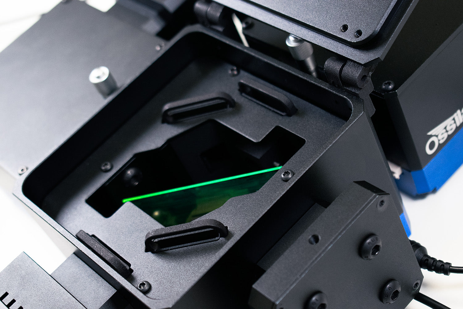
Measuring fluorescence with the Ossila Spectrofluorometer
Measuring Fluorescence
In fluorescence spectroscopy, high energy light from an excitation source, such as UV light source or laser, is directed towards your sample. The sample absorbs this light, exciting all available electrons into their higher energy state.
Then, any emitted light (fluorescence) is collected and analyzed by a detector, noting both the intensity and wavelength. Studying this fluorescence will give you insights into the composition, structure, and behavior of your sample.
Spectrofluorometer components diagram
Measuring fluorescence spectroscopy requires four main components, often integrated into a standalone system:
An Excitation Source
This is often a high energy light source or laser. Your excitation wavelength must be equal to or below the excitation wavelength of your material. There are multiple types of light sources that you can use for fluorescence spectroscopy, including diode lasers and UV LED lights. The type of light source required will depend on your sample, the type of fluorescence you wish to conduct and practical matters such as size, price and safety. Since a fluorophores emission spectrum doesn’t depend on excitation wavelength, a UV light source is high energy enough that it can excite most fluorophores.
You can also use a tunable light source. These sources combine a monochromator with a white light source, allowing you to select an appropriate excitation wavelength for your sample. Alternatively, you can select an excitation wavelength using a white light source and simple filters.
A Detector
Spectrofluorometers use photomultipliers, photodiodes or avalanche photodiodes. These single element detectors can measure light intensity with varying degrees of sophistication. Some detectors are sensitive enough to count individual photons, or to work out quantum efficiency exactly.
A single element detector must be used with a monochromator or filters in order to separate light into its individual wavelengths. The spectrofluorometer will measure intensity at each wavelength, building a spectrum piece by piece.
You can also measure fluorescence using charge couple device detectors, such as those found in UV-vis spectrometers (like the Ossila USB Spectrometer). These systems measure the intensity of all wavelengths at once. This measurement will be much quicker than spectrofluorometers, but will have much lower resolution.
Filters or Monochromators
Ideally, for fluorescence spectroscopy you want to select both your excitation and emission wavelength independently. This can negate effects like Tyndall scattering and ensure you are measuring only what you want to measure. In theory, you could use filters to do this, but taking a whole spectrum becomes a long, difficult process.
A monochromator contains a rotating diffraction grating and a series of adjustable slits to select the wavelength of light that is exposed to the detector. This allows to you track emitted intensity at a specific wavelength or build a fluorescence spectrum while omitting the excitation wavelength from the measurement. Most spectrofluorometers come with two monochromators to enable both absorbance and fluorescence measurements.
Sample Holder and Light Controlling Optics
For accurate and repeatable fluorescence spectroscopy, it is important to ensure consistent placement and alignment of both incident and emitted light within the spectrofluorometer. For this reason, sample holders are usually held in a fixed position within the spectrofluorometer. Fluorescence should always be collected at right angles to the excitation light source
Sometimes, a reference channel is included in the spectrofluorometer design. This will account for time fluctuations of the lamp, and allows for any corrections to be made after measurement. Additionally, all components should be enclosed in a sealed unit or held in place using an optical breadboard.
Fluorescence intensity varies depending on several measurement and instrumental factors including observation geometry, the transmission efficiency of the monochromators and the width of monochromator slits. Because of this its important that correction of spectra is considered for both quantitative and comparative measurement.
Steady State Vs. Time Resolved Fluorescence
Steady-state fluorescence spectroscopy measures fluorescence under constant excitation. This can be used to measure unchanging characteristics about a material including spectral characteristics and relative quantum yields of fluorescent samples.
In contrast, time-resolved fluorescence spectroscopy is used to measure fluorescence lifetime and other dynamic processes like energy transfer, quenching, or environmental interactions,. It measures fluorescence intensity decay after a brief excitation pulse.
To conduct time-resolved measurements, more advanced instrumentation is required, including pulsed light sources (such as lasers or LEDs), fast timing electronics, and high-speed detectors. These setups often involve time-correlated single photon counting (TCSPC) or streak cameras and demand careful control of ambient light, often in a dark-room environment. Examples of time-resolved fluorescence measurements include pulse fluorometry or phase modulation fluorometer .
While steady-state measurements are routine in many labs using standard spectrofluorometers, time-resolved setups are more specialized and typically used in research-intensive environments.
Excitation vs Emission Spectroscopy
In an emission spectrum, you measure variations in fluorescence intensity (IF) at various fluorescence wavelengths (λF). In this measurement, the excitation wavelength (λE) is fixed. This measurement shows the wavelengths where fluorescence is emitted most strongly.
Emission measurements require a high energy light source and a monochromator between the sample and detector to omit the excitation wavelength and vary the measured wavelength.
Excitation measurements track variations in IF at a fixed emission wavelength (λF) and the excitation wavelength is varied. This will show the wavelengths where fluorescence is stimulated most strongly.
Excitation measurements require broadband light source and a monochromator positioned between the light source and the sample.
It is important to note that an excitation spectra is different to absorbance spectra, although they often look similar. The main difference between absorbance and excitation is how they’re measured:
Absorbance measurement use transmitted light. Light is passed through a sample and the intensity of light at different wavelengths is measured relative to the initial intensity. This is often measured by a USB spectrometer, but can also be measured with a spectrofluorometer.
Excitation measurements measure fluorescence at a specific wavelengths. Various wavelengths of light are used to excite the sample, and you measure the fluorescence intensity at a specific wavelength. This measurement requires a spectrofluorometer, it can’t be measured with a simple USB spectrometer.
In some cases, these will look similar because it’s likely that fluorescence intensity will be highest at the wavelengths where photons are most strongly absorbed.
Applications of Fluorescence Spectroscopy
Fluorescence spectroscopy is used in many different industries to do chemical and biological analysis of organic materials. Materials that exhibit fluorescent behavior include:
Materials used in TADF-OLEDs, OLEDs, and OPVs/PSCs
Semiconductor devices themselves such as solar cells and organic light emitting diodes
Quantum dots or nanodots (such as carbon nanodots and perovskite quantum dots)
You can also use fluorescence spectroscopy to track biological processes via Förster resonance energy transfer between fluorophores. Alternatively, fluorescence microscopy can be used to monitor changes in conjugated systems or organic compounds over time or due to changes in environment (solvent, molecular structure, pH, temperature, etc).
The Ossila Spectrofluorometer measures the fluorescence emission spectra of materials with high sensitivity and precision. The spectrofluorometer can take both excitation and emission measurements with the free Spectrophotometry software.
Photoluminescence occurs when electrons radiatively relax from their photoexcited states. Emissions resulting from singlet-singlet transitions are known as fluorescence, however, there are a number of ways in which electrons in these excited states can relax non-radiatively. These are known collectively as fluorescence quenching.
J. R. Lakowicz (2006). Principles of Fluorescence Spectroscopy. (Third Edition) Spinger Science+Business Media. DOI:10.1007/978-0-387-46312-4
B. Valeur (2001). Molecular Fluorescence: Principles and Applications. Wiley-VCH Verlag GmbH. ISBN: 3-527-60024-8
We use essential cookies for core website functionality and collect anonymous, cookieless usage statistics. You can optionally allow analytics cookies to help us improve our site (more information)
Change Country
Change Currency
We were unable to change your currency due to a corrupted or expired cart cookie.
Click continue to delete your cart cookie and change your currency. This will remove all items from your cart. If this fails, please delete all cookies and try again, or contact us for further assistance.


 Measuring Fluorescence with the Ossila Spectrofluorometer
 Fluorescence Quenching and Non-Radiative Relaxation