Python for Spectroscopy: Spectra Data Visualization

Often when working with optical spectroscopy data, data processing can be made faster and more consistent using a programming tool such as Python. These are the steps that our researchers follow when processing multiple spectra that were taken using the Ossila USB Spectrometer. The code was designed in the Spyder virtual environment for Python but should be compatible with other environments such as Jupyter Notebooks. This code is designed for the Ossila Optical Spectrometer but could be adapted to process data from other spectrometers as long as the data is in the form of a CSV.
When Taking the Measurements
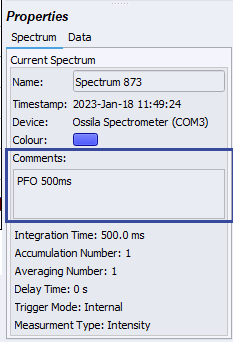
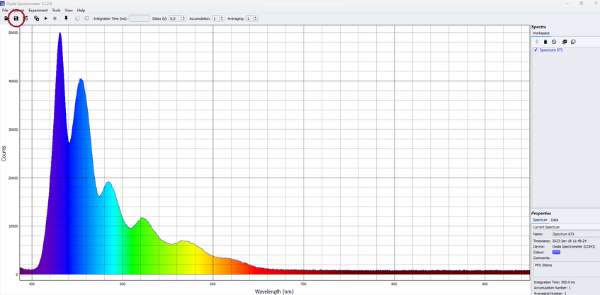
First, capture the spectrum produced by your sample using the Single Shot Data Acquisition function in the Ossila Optical Spectrometer Software (the play button on the top left of the window). To name your spectra, enter the sample label into the "Comments" box of the Ossila Optical Spectrometer Software. This will help keep track of what sample relates to which spectra - and will be useful in the code later on.
Once this is taken, ensure the spectra you want to save are checked on the workspace toolbar on the right-hand side. Then, save this spectrum using the "Save" icon on the top left of the window, or by selecting File -- Save Checked Spectra. This will open a new window where you can choose where to save the files to. If you wish to compare measurements using this method, make sure all these spectra are within the same file.
When you save a measurement from the Ossila USB Spectrometer, it will save as a CSV code in the following format.
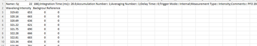
This CSV file contains all the experimental details about the measurement you have taken (integration time, number of spectral averages, measurement type) as well as your actual data.
However, when comparing multiple spectra, it can be a pain to manually extract data from each individual CSV file. Using a data processing tool such as python can really save you some time and energy in data processing, without placing limits on the adaptability of your experimental set up.
Plotting The Data
The benefit of using a programming language for data presentation is that you are processing all your data in the same way. Additionally, data presentation and processing parameters can be personalised to suit your preference or experimental specifications. Also, most importantly, it is a lot quicker and easier! We have written a basic Python script which you can use to quickly plot multiple spectra from the Ossila Optical Spectrometer.
This code was written in Spyder but this should also work for other Python environments like Jupyter Notebook. We have split the sections of code into different cells which you should run in this order. In Spyder, "#%%" is used to split sections of code into separate cells, so these have been included in the code we provide.
You should start by importing the necessary packages into your Python environment. Some of these packages are included when you download Python, but some may need to be installed using the package installer for python (pip).
# Import the following packages
# These packages are included with Python
import csv
from pathlib import Path
from tkinter import Tk
from tkinter import filedialog
# These packages need to be installed using pip
import matplotlib.pyplot as plt
import pandas as pd
Then, define a function to plot the data for you. The plot_spectra function below takes a CSV file produced from an Ossila Optical Spectrometer and plots it onto a single axes using panda DataFrame.
#%%
# This function plots Wavelength vs. Intensity from a Ossila Optical Spectrometer csv file.
def plot_spectra(file_path, labels, index):
"""Plot Wavelength vs. Intensity from an Ossila Optical Spectrometer csv file."""
# Read information from a CSV file into a DataFrame
data = pd.read_csv(file_path, skiprows=1, engine='python')
# Plot Wavelength vs. Intensity
data.set_index('Wavelength (nm)', inplace=True)
data['Intensity'].plot(label=labels[index])
Next, define a function to extract the experimental details about the measurement. This can be important information to store for future reference or for data analysis.
#%%
# This function will extract the experimental details about an Ossila measurement CSV file into a DataFrame.
# It returns a DataFrame containing all the experimental information.
def get_spectral_info(file_path) -> pd.DataFrame:
"""Extract experimental details from an Ossila file into an DataFrame."""
# Open and read CSV file
with file_path.open('r', newline='') as in_file:
reader = csv.reader(in_file)
# Extract experimental information from the first row into a single string
for i, row in enumerate(reader):
if i == 0:
information = f'{row[0]} {row[1]}{row[2]}'
else:
break
# Split the string into its component parts, and put into a DataFrame
df = pd.DataFrame([x.split('::') for x in information.split(';')])
df = df.transpose()
# Grab the first row for headers for column heads
df.columns = df.iloc[0]
df = df[1:]
# A few small formatting steps to make the DataFrame more readable
df.set_index('Name', inplace=True)
return df
Once these functions are defined, we want to choose the files we want to look at using the Tkinter package.
#%%
# Here we use Tkinter to make a list of CSV files we want to look at
master = Tk()
file_list = filedialog.askopenfilenames()
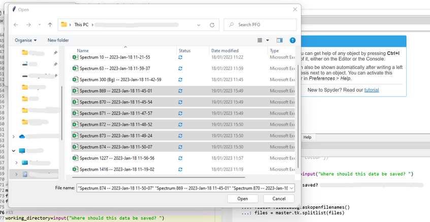
Running this code will open a new window. In this window, you can locate and select the files you want to look at. Click open to load these.
Tkinter functionThere are many parts to the above cell, but these are the "main steps" taken to process the data. However, the output should be a graph plotting all the desired spectra, and a DataFrame called spectral_information containing the experimental details about each measurement.
#%%
# This cell extracts the information from all the csv files in 'file_list'
# Define an empty DataFrame for the experimental details
spectral_information = []
spectral_information = pd.DataFrame(spectral_information)
# Run each csv file in the 'file_list' list through get_spectral_info() and plot_spectra()
for i, file_path in enumerate(file_list):
# Skip the file if it is not a csv file
file_path = Path(file_path)
if file_path.suffix != '.csv':
continue
# Extract experimental details into the DataFrame, spectral_information
data = get_spectral_info(file_path)
spectral_information = pd.concat(spectral_information , data)
# Add the wavelength-intensity plot for each measurement to a single set of axes
# Each spectrum will be labeled with the name given in the comments
labels = spectral_information['Comments']
plot_spectra(file_path, labels, i)
# This sets qualities about graph plotted, such as the x-axis and y-axis range
# For more personalisation or to change graph presentation, see MatPlotLib's documentation
plt.xlim(360, 900)
plt.legend(ncol=2)
# If 'Y' or 'y' is entered, this will save the graph as a png, and the DataFrame as a csv
save_output = input('Do you want to save this graph? (Y/N)\n')
if save_output in ['Y', 'y']:
# Enter the directory where you want to store your saved data
# This will keep asking until you input a working_directory
working_directory = ''
while not working_directory:
working_directory = input('Where should this data be saved?\n')
working_directory = Path(working_directory)
# Enter a name for the file into input window
save_name = input('What do you want to save this as?\n')
plt.savefig(
working_directory / f'{save_name}.png',
transparent=False,
bbox_inches='tight',
dpi=300,
)
spectral_information.to_csv(working_directory / f'{save_name}.csv')
plt.show()
An input line will also appear asking you if you want to save the spectra. Enter "Y" or "y" (no spaces) if you wish to save the graph and DataFrame as a .png and .csv file respectively. You should then be presented with two more input lines asking you where you want the data to be saved, and under what name. Enter the desired pathway and file name for each input line, and press enter to save this. An example figure produced using this code is shown below. This shows the fluorescence from PFO films measured for varying integration times (in milliseconds).

Module List
Details and licensing information on of the modules used in this code is provided below.
Matplotlib
Matplotlib is a library that is used in Python to easily create a display various forms of charts and graphs. Plotting is as simple as calling plot(x_values, y_values) in most cases. More can be seen in our tutorials on matplotlib.
Pandas
Pandas is a python package that simplifies working with "labeled" or "relational" data, making real-world data analysis faster and easier. Processing files using DataFrames can make data handling, plotting and analyzing uncomplicated and simple.
Full Code
# Import the following packages
# These packages are included with Python
import csv
from pathlib import Path
from tkinter import Tk
from tkinter import filedialog
# These packages need to be installed using pip
import matplotlib.pyplot as plt
import pandas as pd
#%%
def plot_spectra(file_path, labels, index):
"""Plot Wavelength vs. Intensity from an Ossila Optical Spectrometer csv file."""
# Read information from a CSV file into a DataFrame
data = pd.read_csv(file_path, skiprows=1, engine='python')
# Plot Wavelength vs. Intensity
data.set_index('Wavelength (nm)', inplace=True)
data['Intensity'].plot(label=labels[index])
#%%
def get_spectral_info(file_path) -> pd.DataFrame:
"""Extract experimental details from an Ossila file into an DataFrame."""
# Open and read CSV file
with file_path.open('r', newline='') as in_file:
reader = csv.reader(in_file)
# Extract experimental information from the first row into a single string
for i, row in enumerate(reader):
if i == 0:
information = f'{row[0]} {row[1]}{row[2]}'
else:
break
# Split the string into its component parts, and put into a DataFrame
df = pd.DataFrame([x.split('::') for x in information.split(';')])
df = df.transpose()
# Grab the first row for headers for column heads
df.columns = df.iloc[0]
df = df[1:]
# A few small formatting steps to make the DataFrame more readable
df.set_index('Name', inplace=True)
return df
#%%
# Here we use TkInter to make a list of CSV files we want to look at
master = Tk()
file_list = filedialog.askopenfilenames()
#%%
# This cell extracts the information from all the csv files in 'file_list'
# Define an empty DataFrame for the experimental details
spectral_information = []
spectral_information = pd.DataFrame(spectral_information)
# Run each csv file in the 'file_list' list through get_spectral_info() and plot_spectra()
for i, file_path in enumerate(file_list):
# Skip the file if it is not a csv file
file_path = Path(file_path)
if file_path.suffix != '.csv':
continue
# Extract experimental details into the DataFrame, spectral_information
data = get_spectral_info(file_path)
spectral_information = spectral_information.append(data)
# Add the wavelength-intensity plot for each measurement to a single set of axes
# Each spectrum will be labeled with the name given in the comments
labels = spectral_information['Comments']
plot_spectra(file_path, labels, i)
# This sets qualities about graph plotted, such as the x-axis and y-axis range
# For more personalisation or to change graph presentation, see MatPlotLib's documentation
plt.xlim(360, 900)
plt.legend(ncol=2)
# If 'Y' or 'y' is entered, this will save the graph as a png, and the DataFrame as a csv
save_output = input('Do you want to save this graph? (Y/N)\n')
if save_output in ['Y', 'y']:
# Enter the directory where you want to store your saved data
working_directory = ''
while not working_directory:
working_directory = input('Where should this data be saved?\n')
working_directory = Path(working_directory)
# Enter a name for the file into input window
save_name = input('What do you want to save this as?\n')
plt.savefig(
working_directory / f'{save_name}.png',
transparent=False,
bbox_inches='tight',
dpi=300,
)
spectral_information.to_csv(working_directory / f'{save_name}.csv')
plt.show()
USB Spectrometer

Learn More
 What Can Absorbance Measurements Tell You?
There are so many material properties that you can measure with this technique. Additionally, the amount of information you can gain from these readings will depend entirely on your sample.
Read more...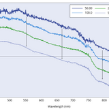 Negative Absorbance: Can Absorbance Ever Be Negative?
In general, you should not be measuring negative absorbance values for any sample.
Read more...