Contact Angle Goniometer User Manual
1. Overview
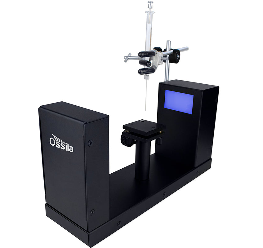
The Ossila Contact Angle Goniometer, part of the Institute of Physics award-winning Solar Cell Prototyping Platform*, provides a fast, reliable, and easy method to measure the contact angle or surface tension of a droplet. The system comes complete with PC software that provides a simple and intuitive interface for contact angle measurements.
2. EU Declaration of Conformity (DoC)
We
Company Name: Ossila BV
Postal Address: Biopartner 3 Building, Galileiweg 8
Postcode: 2333 BD Leiden
Country: The Netherlands
Telephone Number: +31 (0)718 081020
Email Address: info@ossila.com
declare that the DoC is issued under our sole responsibility and belongs to the following product:
Product: Contact Angle Goniometer (L2004A1)
Serial Number: L2004A1 - xxxx
Object of Declaration
Contact Angle Goniometer (L2004A1)
The object of declaration described above is in conformity with the relevant Union harmonization legislation:
EMC Directive 2014/30/EU
RoHS Directive 2011/65/EU
Signed:
Name: Dr James Kingsley
Place: Leiden
Date: 16/11/2021
| Декларация | за съответствие на ЕС |
|---|---|
| Производител | Ossila BV, Biopartner 3 building, Galileiweg 8, 2333 BD Leiden, NL. |
| Декларира с цялата си отговорност, че посоченото оборудване съответства на приложимото законодателство на ЕС за хармонизиране, посочено на предходната(-ите) страница(-и) на настоящия документ. | |
| [Čeština] | Prohlášení o shodě EU |
|---|---|
| Výrobce | Ossila BV, Biopartner 3 building, Galileiweg 8, 2333 BD Leiden, NL. |
| Prohlašujeme na vlastní odpovědnost, že uvedené zařízeni je v souladu s příslušnými harmonizačními předpisy EU uvedenými na předchozích stranách tohoto dokumentu. | |
| [Dansk] | EU-overensstemme lseserklærin g |
|---|---|
| Producent | Ossila BV, Biopartner 3 building, Galileiweg 8, 2333 BD Leiden, NL. |
| Erklærer herved, at vi alene er ansvarlige for, at det nævnte udstyr er i overensstemmelse med den relevante EUharmoniseringslovgivning, der er anført på den/de foregående side(r) i dette dokument. | |
| [Deutsch] | EU-Konformitätserklärung |
|---|---|
| Hersteller | Ossila BV, Biopartner 3 building, Galileiweg 8, 2333 BD Leiden, NL. |
| Wir erklären in alleiniger Verantwortung, dass das aufgeführte Gerät konform mit der relevanten EUHarmonisierungsgesetzgebung auf den vorangegangenen Seiten dieses Dokuments ist. | |
| [Eesti keel] | ELi vastavusavaldus |
|---|---|
| Tootja | Ossila BV, Biopartner 3 building, Galileiweg 8, 2333 BD Leiden, NL. |
| Kinnitame oma ainuvastutusel, et loetletud seadmed on kooskõlas antud dokumendi eelmisel lehelküljel / eelmistel lehekülgedel ära toodud asjaomaste ELi ühtlustamise õigusaktidega. | |
| [Ελληνικά] | Δήλωση πιστότητας ΕΕ |
|---|---|
| Κατασκευαστής | Ossila BV, Biopartner 3 building, Galileiweg 8, 2333 BD Leiden, NL. |
| Δηλώνουμε υπεύθυνα όn ο αναφερόμενος εξοπλισμός συμμορφώνεται με τη σχεnκή νομοθεσία εναρμόνισης της ΕΕ που υπάρχει σnς προηγούμενες σελίδες του παρόντος εγγράφου. | |
| [Español] | Declaración de conformidad UE |
|---|---|
| Fabricante | Ossila BV, Biopartner 3 building, Galileiweg 8, 2333 BD Leiden, NL. |
| Declaramos bajo nuestra única responsabilidad que el siguiente producto se ajusta a la pertinente legislación de armonización de la UE enumerada en las páginas anteriores de este documento. | |
| [Français] | Déclaration de conformité UE |
|---|---|
| Fabricant | Ossila BV, Biopartner 3 building, Galileiweg 8, 2333 BD Leiden, NL. |
| Déclarons sous notre seule responsabilité que le matériel mentionné est conforme à la législation en vigueur de l'UE présentée sur la/les page(s) précédente(s) de ce document. | |
| [Hrvatski] | E.U izjava o sukladnosti |
|---|---|
| Proizvođač | Ossila BV, Biopartner 3 building, Galileiweg 8, 2333 BD Leiden, NL. |
| Izjavljujemo na vlastitu odgovornost da je navedena oprema sukladna s mjerodavnim zakonodavstvom EU-a o usklađivanju koje je navedeno na prethodnoj(nim) stranici(ama) ovoga dokumenta. | |
| [Italiano] | Dichiarazione di conformità UE |
|---|---|
| Produttore | Ossila BV, Biopartner 3 building, Galileiweg 8, 2333 BD Leiden, NL. |
| Si dichiara sotto la propria personale responsabilità che l'apparecchiatura in elenco è conforme alla normativa di armonizzazione UE rilevante indicata nelle pagine precedenti del presente documento. | |
| [Latviešu] | ES atbils tības deklarācija |
|---|---|
| Ražotājs | Ossila BV, Biopartner 3 building, Galileiweg 8, 2333 BD Leiden, NL. |
| Ar pilnu atbilclību paziņojam, ka uzskaitītais aprīkojums atbilst attiecīgajiem ES saskaņošanas tiesību aktiem, kas minēti iepriekšējās šī dokumenta lapās. | |
| [Lietuvių k.] | ES atitikties deklaracija |
|---|---|
| Gamintojas | Ossila BV, Biopartner 3 building, Galileiweg 8, 2333 BD Leiden, NL. |
| atsakingai pareiškia, kad išvardinta įranga atitinka aktualius ES harmonizavimo teisės aktus, nurodytus ankstesniuose šio dokumento | |
| [Magyar] | EU-s megfelelőségi nyilatkozat |
|---|---|
| Gyártó | Ossila BV, Biopartner 3 building, Galileiweg 8, 2333 BD Leiden, NL. |
| Kizárólagos felelösségünk mellett kijelentjük, hogy a felsorolt eszköz megfelel az ezen dokumentum előző oldalán/oldalain található EU-s összehangolt jogszabályok vonatkozó rendelkezéseinek. | |
| [Nederlands] | EU-Conformiteitsverklaring |
|---|---|
| Fabrikant | Ossila BV, Biopartner 3 building, Galileiweg 8, 2333 BD Leiden, NL. |
| Verklaart onder onze uitsluitende verantwoordelijkheid dat de vermelde apparatuur in overeenstemming is met de relevante harmonisatiewetgeving van de EU op de vorige pagina('s) van dit document. | |
| [Norsk] | EU-samsvarserklæ ring |
|---|---|
| Produsent | Ossila BV, Biopartner 3 building, Galileiweg 8, 2333 BD Leiden, NL. |
| Erklærer under vårt eneansvar at utstyret oppført er i overholdelse med relevant EU-harmoniseringslavverk som står på de(n) forrige siden(e) i dette dokumentet. | |
| [Polski] | Deklaracja zgodności Unii Europejskiej |
|---|---|
| Producent | Ossila BV, Biopartner 3 building, Galileiweg 8, 2333 BD Leiden, NL. |
| Oświadczamy na własną odpowiedzialność, że podane urządzenie jest zgodne ze stosownymi przepisami harmonizacyjnymi Unii Europejskiej, które przedstawiono na poprzednich stronach niniejszego dokumentu. | |
| [Por tuguês] | Declaração de Conformidade UE |
|---|---|
| Fabricante | Ossila BV, Biopartner 3 building, Galileiweg 8, 2333 BD Leiden, NL. |
| Declara sob sua exclusiva responsabilidade que o equipamento indicado está em conformidade com a legislação de harmonização relevante da UE mencionada na(s) página(s) anterior(es) deste documento. | |
| [Română] | Declaraţie de conformitate UE |
|---|---|
| Producător | Ossila BV, Biopartner 3 building, Galileiweg 8, 2333 BD Leiden, NL. |
| Declară pe proprie răspundere că echipamentul prezentat este în conformitate cu prevederile legislaţiei UE de armonizare aplicabile prezentate la pagina/paginile anterioare a/ale acestui document. | |
| [Slovensky] | Vyhlásenie o zhode pre EÚ |
|---|---|
| Výrobca | Ossila BV, Biopartner 3 building, Galileiweg 8, 2333 BD Leiden, NL. |
| Na vlastnú zodpovednosť prehlasuje, že uvedené zariadenie je v súlade s príslušnými právnymi predpismi EÚ o harmonizácii uvedenými na predchádzajúcich stranách tohto dokumentu. | |
| [Slovenščina] | Izjava EU o skladnosti |
|---|---|
| Proizvajalec | Ossila BV, Biopartner 3 building, Galileiweg 8, 2333 BD Leiden, NL. |
| s polno odgovornostjo izjavlja, da je navedena oprema skladna z veljavno uskladitveno zakonodajo EU, navedeno na prejšnji strani/prejšnjih straneh tega dokumenta. | |
| [Suomi] | EU-vaatimustenm ukaisuusvakuutus |
|---|---|
| Valmistaja | Ossila BV, Biopartner 3 building, Galileiweg 8, 2333 BD Leiden, NL. |
| Vakuutamme täten olevamme yksin vastuussa siitä, että tässä asiakirjassa luetellut laitteet ovat tämän asiakirjan sivuilla edellisillä sivuilla kuvattujen olennaisten yhdenmukaistamista koskevien EU-säädösten vaatimusten mukaisia. | |
| [Svenska] | EU-försäkran om överensstämmelse |
|---|---|
| Tillverkare | Ossila BV, Biopartner 3 building, Galileiweg 8, 2333 BD Leiden, NL. |
| Vi intygar härmed att den utrustning som förtecknas överensstämmer med relevanta förordningar gällande EUharmonisering som fmns på föregående | |
3. Safety
3.1 Warning
To avoid safety hazards, obey the following:
- Do not look directly into the backlight.
- Turn the backlight of when the system is not in use.
3.2 Caution
- Only use the device for the purposes intended (described in this document).
- Take care when handling syringes to avoid touching the needle tip.
- If using within a shared workspace, position the backlight to point away from others.
- Take care to avoid trapping fingers while adjusting the tilt stage position.
4. Requirements
Table 4.1 details the power requirements for the system, and the minimum computer specifications for the Ossila Contact Angle software.
Table 4.1 Contact Angle Goniometer and Contact Angle software requirements.
| Power | 24 VDC |
|---|---|
| Operating Systems | Windows 10 or 11 (32-bit or 64-bit) |
| CPU | Quad Core 2.5 GHz |
| RAM | 2 GB |
| Available Hard Disk Space | 207 MB |
| Monitor Resolution | 1920 x 1080 |
| Connectivity | USB 2.0 (The USB connection does not supply power to the backlight) |
5. Unpacking
5.1 Packing List
The standard items included with the Ossila Contact Angle Goniometer are:
- The Ossila Contact Angle Goniometer.
- Tilt stage assembly.
- Microlitre syringe.
- 10 mm diameter calibration sphere.
- 24 VDC power adapter.
- USB-A to USB-B cable.
- USB memory stick pre-loaded with the user manual and software installer.
5.2 Damage Inspection
Examine the components for evidence of shipping damage. If damage has occurred, please contact Ossila directly for further action. The shipping packaging will come with a shock indicator to show if there has been any mishandling of the package during transportation.
6. Specifications
The Contact Angle Goniometer measurement specifications are shown in Table 6.1, and the physical specifications are shown in Table 6.2.
Table 6.1 Contact Angle Goniometer measurement specifications
| Angle range | 5° to 180° |
|---|---|
| Max measurement speed | 33 ms (30 fps) |
Table 6.2 Contact Angle Goniometer physical specifications
| Stage Dimensions | 50 mm x 50 mmm |
|---|---|
| Maximum Droplet Width | 20 mm |
| Overall Product Dimensions |
Width: 95 mm Height: 170 mm Depth: 320 mm |
| Maximum Sample Thickness | 20 mm |
| Maximum Camera Resolution | 1920 x 1080 |
7. Installation
- Connect the system to your computer using the USB cable provided.
- Plug in the power adapter, connect it to the unit, and check that the backlight turns on.
- Run the file ‘Ossila-Contact-Angle-Installer-4-x-x-x.exe’ on the USB drive provided and follow the on-screen instructions to install the Contact Angle Software.
8. Operation
8.1 Recording a Video
Video recording is performed in the ‘Camera View Finder’ window which can be opened by clicking the camera button located in the top left of the software.
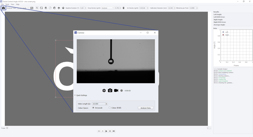
To record a video or an image, follow the instructions below. For more detailed information on individual settings, see Section 8.2.
- Open the Ossila Contact Angle software.
- Click the ‘Camera’ icon. The camera view finder should appear in the middle of the screen.
- Place your sample in the center of the vertical tilt stage.
- Adjust the stage height until sample can be seen in the bottom half of the image.
- Twist the camera lens until the sample is in focus on the display.
- To change the default video settings, click the settings or ‘Cog’ icon or expand the quick settings.
- Set a recording duration (video length) and speed (frame rate). Make sure that your video length accounts for the time it will take to dispense the droplet and any spreading time that you wish to observe.
- Prepare to dispense a droplet.
- Click the ‘Camera’ or ‘Record’ icon to capture.
- Dispense the droplet.
- When you are finished taking recordings, press ‘Stop Camera’ to turn the camera off.
8.2 Software Settings
8.2.1 Camera Quick Settings
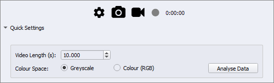
(I) Video Length
Sets the total length of time to record for.
Choose a number between 0.1 and 3600 seconds. The default value is 10 seconds
(II) Color Space
Determines whether the captured videos and images are greyscale (black/white) or colored.
(III) Analyze Data
Send the last captured video or image to the analysis view.
8.2.2 Recording Settings
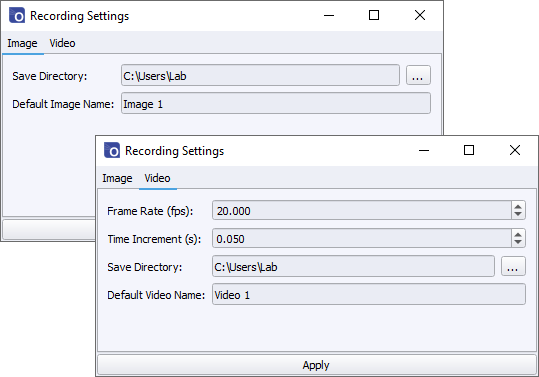
(I) Frame Rate
Sets the frame rate in frames per second. This will update the increment to match the chosen frame rate, the default value is 20 frames per second.
(II) Time Increment
Sets the time increment in seconds. This will update the frame rate to match the chosen increment, the default value is 0.05 seconds.
(III) Save Directory
Sets the directory in which images and videos are saved. This can be input manually or selected using the button with the ellipsis.
(IV) Default Video/Image Name
Sets the name ofthe video/image file. If a file with the same name is saved, a number will be included in the file name so that the original file is not overwritten
Video files are saved as .avi files. Image files are saved as .png files.
8.3 Performing Measurements
Both contact angle and surface tension measurements are performed in the main window by clicking the ‘Analyze’ icon.
To perform contact angle or surface tension measurements, follow the instructions in Sections 8.3.1 or 8.3.2 respectively. For more detailed information on individual settings, please see later in this section.
8.3.1 Contact Angle Measurements
- In the file menu, select ‘Load’ icon (Ctrl + L)
- Use the file dialogue to select a video or image for analysis. The name of the selected video will be displayed in the window title.
- The selected video or image will be displayed in the center of the screen.
- Select ‘Contact Angle’ as the measurement choice in the analysis type drop down menu.
- Use the video controls beneath the display to navigate to a frame that has a droplet.
- Adjust the region of interest (ROI) box until the entire droplet is within the box.
- The baseline of the measurement is the bottom of the ROI box.
- Make sure that the bottom line is level with the base of the droplet.
- If the image is slanted, or the stage was not completely level, you can adjust the baseline angle using the ‘Baseline Rotation’ box in the top right corner.
- Fine adjustments to the baseline height can be made using the up and down arrows in the top right corner.
- Click ‘Analyze’.
- The software will detect the edges of the droplet within the ROI.
- A fitting technique is applied to the droplet, depending on its estimated angle:
- < 10°: Circle Fit
- > 10°: Polynomial Fit
- The gradient of the fit at the baseline is used to calculate the contact angle.
- Click the play button (optional).
- The program will cycle through the frames in the video and fit a contact angle to the droplet in each frame.
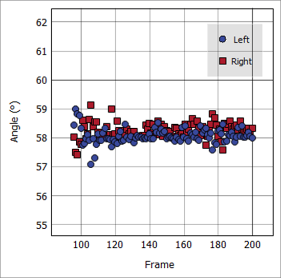
- The calculated angles are displayed in the left corner of the screen as a contact angle vs frame plot.
Choose a directory in ‘File’ –> ‘Select save directory’ and save the results by clicking the ‘Save Analysis’ icon (Ctrl + S).
The results are saved in a comma separated values (.csv) file, which can easily be opened in any data analysis program.
8.3.2 Surface Tension Measurements
- In the 'File’ menu, select ‘Load’ (Ctrl + L)
- Use the file dialogue to select a video or image for analysis. The name of the selected file is then displayed in the window title at the top of the software.
- The video or image will be displayed in the center of the screen.
- Select a drop density. If the liquid is not in the drop-down list, select ‘Add New’ to add a new liquid to the settings.
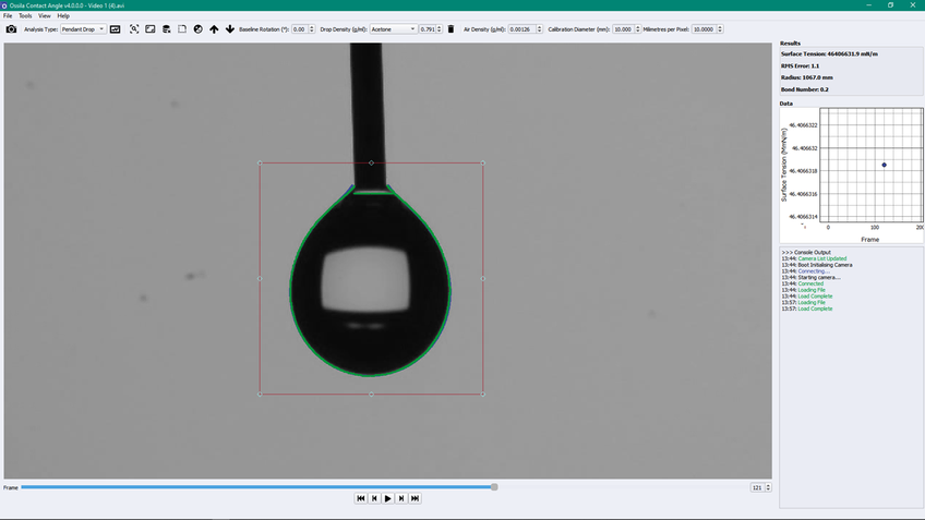
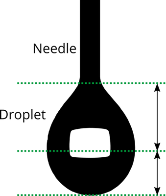
- Use the video controls beneath the display to navigate to a frame that has a suitable droplet. The droplet should be pushed out of the needle tip until it is close to falling.
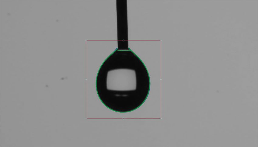
- Adjust the region of interest (ROI) box until the entire droplet and the very bottom of the needle is within the box (as shown in Figure 8.6). If the image is slanted, you can adjust the image angle using the ‘Baseline Rotation’ box in the top right corner.
- Click ‘Analyze’.
- The software will detect the edges of the droplet within the ROI.
- A fitting technique is applied to the droplet. The parameters of the fit (radius, B number, X0, Y0) are shown in the top right of the viewing window.
- The calculated surface tension is displayed in the left corner of the screen.
- Choose a directory in File – Select save directory and save the results by clicking the ‘Save Analysis’ icon (Ctrl + S). The results are saved in a comma separated values (.csv) file, which can easily be opened in any data analysis program.
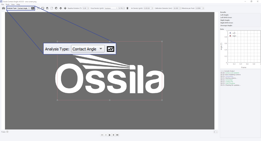
8.3.3 Analysis Control
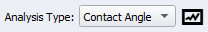
(I) Analysis Type
Choose either Contact Angle or Pendant Drop. This will affect which measurement is performed when the ‘Analyze’ button is pressed.
(II) Analyze
Performs the chosen analysis type on the image within the region of interest box. The resultant fits are shown on the image and the calculated contact angles, or surface tension measurements are displayed in the results display.
8.3.4 Solvent Type Selection

(I) Drop Density (Pendant Drop Only)
Select the drop density of the liquid under investigation. This density is used along with the droplet fitting to determine the surface tension. If a suitable density is not in the list, select ‘Add New’. The new density will be saved to file.
Clicking the ‘Delete/Bin’ icon deletes the currently selected solvent.
(II) Air Density (Pendant Drop Only)
This is the density of the air surrounding the droplet. This can be left as the default value in most circumstances.
8.3.5 Calibration Controls
To calibrate the measurement, select calibrate in ‘Tools’ → ‘Calibrate’. This performs the calibration procedure on the calibration sample within the region of interest. For more information on calibration, see Section 9.

(I) Calibration Diameter
Select the diameter of the calibration sample under test.
The calibration sphere provided with the system has a diameter of 10 mm, which is the default value of this field.
(II) Millimeters per Pixel
Shows the millimeters per pixel determined by the calibration procedure.
8.3.6 Results Display
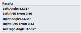
(I) Left Angle, Right Angle
Shows the measured contact angle in the current frame for the left and right sides of the droplet.
(II) Left RMS Error, Right RMS Error, RMS Error
Shows the root-mean-square error of the polynomial fit to the detected edge data.
A fit with an RMS error value greater than or equal to 1 is poor, and the results data is discarded for the corresponding frame.
(III) Average Angle
Shows mean average of the left and right angles.
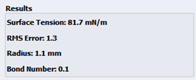
(IV) Surface Tension
Shows the measured surface tension.
(V) Radius
Shows the measured drop radius.
(VI) Bond Number
Shows the measured bond number
8.3.7 Results Plot
Plots the contact angles or surface tensions measured against frame for the currently selected video or image.
8.3.8 Main Viewer/Main Viewer Controls
(I) Main Viewer
Displays the selected video for analysis.
(II) Display Controls
Controls how the image appears in the main viewer.

- Reset Zoom restores the window to its default zoom.
- Reset ROI restores the ROI box to the center of the screen.
- Clear Fit removes the contact angle fit from the viewer.
- Show Edges displays the edge detection used in the contact angle measurement. For more information on the edge detection, see Section 10.3.
- Binary Thresholding turns on binary thresholding.
- and baseline rotation options adjust the height and rotation of the baseline with respect to the main image. The rotation box allows manual editing of the pendant drop fitting parameters
(III) Region of Interest (ROI) Box
Defines the region of interest for the contact angle and surface tension measurements. Only the part of the image inside the box will be used in the analysis. The baseline of the measurement is defined by the bottom of the box.
8.3.9 Video Controls
(I) Frame Controls
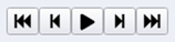
| Button | Function |
|---|---|
| Play (Visible while paused) |
Cycles through every frame in the video. If ‘Contact Angle’ is selected and the ‘Analyze’ button is checked, the contact angle will be measured for each frame whilst playing. |
| Pause (Visible while playing) | If pressed after ‘Play’, the video will stop at the current frame. |
| First | Displays the first frame in the video. |
| Previous | Displays the previous frame in the video |
| Next | Displays the next frame in the video |
| Last | Displays the last frame in the video |
(II) Frame

Displays the index number of the frame being displayed. The first frame in the video has an index of 0.
(III) Video Progress Bar
The video progress bar gives a visual representation of the relative position the frame in the video. The selected frame can also be adjusted using the progress bar.
8.3.10 Saving Data
Results files are saved in a tabular format as comma separated values (.csv) files, which can be opened with most spreadsheet programs. For contact angle analysis, the file contains seven columns of data, which are described in Table 8.1. For surface tension analysis, the file contains 5 columns of data, which are described in Table 8.2. The save directory and file name can be selected using the controls in the file menu.
Table 8.1 Column names and descriptions for contact angle data saved in the results file.
| Column Name | Description |
|---|---|
| Frame Number | The frame number of the video file. |
| Time (s) | The time at the frame number. |
| Left Angle (°) | Left fitted contact angle. |
| Right Angle (°) | Right fitted contact angle. |
| Average Angle (°) | Mean average of the right and left angles. |
| Left Contact Point | The x coordinate (in pixels) at the point where the left edge of the droplet intercepts the baseline. |
| Right Contact Point | The x coordinate (in pixels) at the point where the right edge of the droplet intercepts the baseline. |
| Droplet Width (Pixels) | The difference in pixels between the left and right contact points. |
Table 8.2 Column names and descriptions for surface tension data saved in the results .csv file.
| Column Name | Description |
|---|---|
| Frame Number | The frame number of the video file. |
| Time (s) | The time at the frame number. |
| Surface Tension (mN/m) | Surface Tension in millinewtons per meter. |
| RMSE | Root mean squared fit of the simulated pendant drop to the detected droplet edge. |
| Drop Volume (µL) | Calculated droplet volume of the simulated pendant drop. |
(I) Save Directory (File → Default Save Directory)
Sets the directory in which videos are saved.
Save Results (File → Save Analysis)
Saves the results to file.
9. Calibration
9.1 Calibration Recording
The system is calibrated by focusing on a sphere with a known width. The software detects the edges of the sphere and determines the number of pixels that correspond to the known diameter. The first step in calibration is to record a video or image of the calibration sphere.
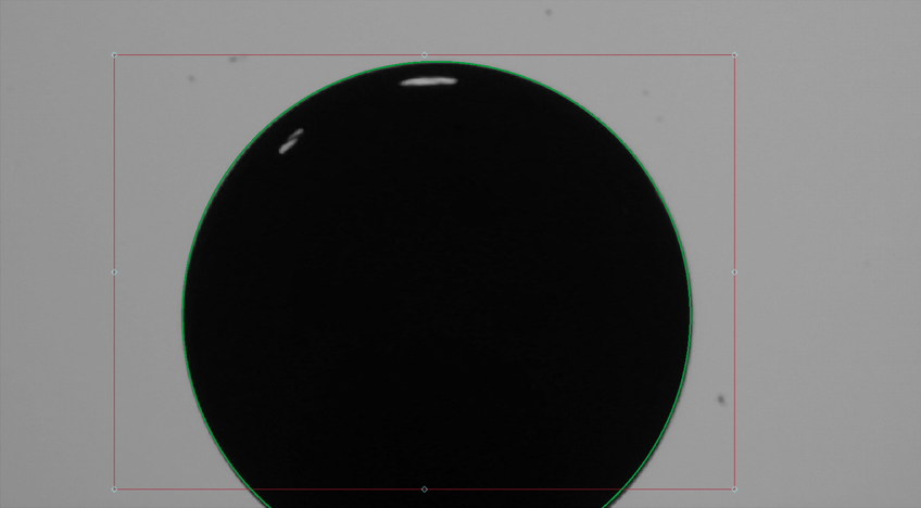
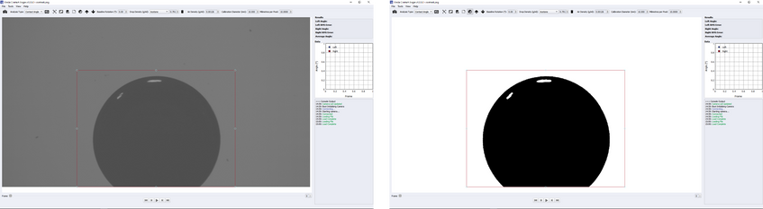
9.2 Calibration Analysis
Once a video or image has been recorded, open it in the ‘Analysis’ tab of the software. Click the ‘Pendant Drop’ option in the top left of the window. Choose the calibration diameter (the calibration sphere provided with the system is 10 mm). Drag the region of interest box so that is surrounds most of the sphere, as shown in Figure 9.1. Click ‘Calibrate’ in ‘Tools’, and the software will fit a circle to the edge of the sphere. This is seen as a green line. The ‘Millimeters per Pixel’ field will update with the new value.
The software will save the new calibration value and it will remain when the software is closed and reopened. If the camera focal distance is changed, the system will need to be re-calibrated.
10. Advanced Measurement Guide
10.1 Region of Interest (ROI)
The region of interest (ROI) is set using the ROI box in the main viewer. Figure 10.1 shows the ROI box as is appears on a droplet image. The box has handles on the sides and corners that can be dragged to resize it. The baseline can be moved pixel-by-pixel using the ‘Baseline Adjustment’ controls in the top right corner of the main viewer.
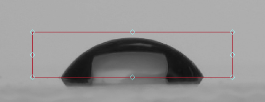
10.1.1 ROI Box Bottom Line (Baseline)
The most important line is the bottom, as this defines the baseline of the measurement. A useful method for determining baseline position is to use the point of reflection of a droplet on a surface. Figure 10.1 shows a droplet reflecting on its substrate. The pointed edges of this droplet are used to position the baseline. Only the part of the image above the baseline will be used in the fitting and resultant contact angle calculations.
10.1.2 ROI Box Top, Left and Right Lines
The top, left, and right sides of the ROI box are used to exclude any unwanted features from the image. If there is a second droplet on the same substrate, this should be excluded from the region of interest.
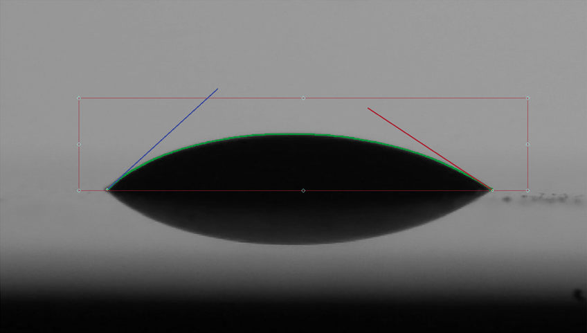
10.2 Polynomial Fitting
If the contact angle is above 10° then the software will fit a polynomial fit to the edge of the droplet. The fit is overlaid on the video or image as shown in Figure 10.2.
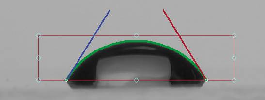
- The green line is the polynomial fit.
- The green dots shows the detected edge (these are more visible when zoomed in to the image).
- The blue line is the left contact angle.
- The red line is the right contact angle.
If the angle is below 10° then the software uses a circle fit to determine the contact angles. This is not displayed on the image.
10.3 Image Processing
10.3.1 Canny Edge Detection
Canny edge detection is the process by which the software determines the edge pixels of a droplet. Figure 10.3 shows the same droplet as Figure 10.1 when the ‘Show Edges’ option has been toggled in the main viewer.
The edge detection algorithm looks for large changes in pixel lightness that would signify the edge of a region of darkness (a droplet). When an area of the image changes from light to dark over a small number of pixels, there is likely to be an edge. Figure 10.4 shows a change in lightness between pixels in a straight line. The pixel on the left has a lightness value of 50, which increases to 240 over the 6 pixels in the line. The change in lightness between the two central pixels is the highest, shown by the steep gradient of the line between these points.

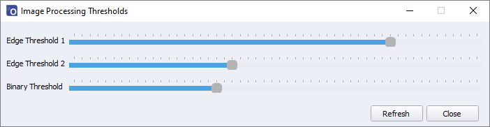
There are two gradient thresholds involved with the edge detection, and they are shown in Figure 10.5. Threshold 1 determines the minimum change in lightness required for an edge to be detected. To detect and edge in Figure 10.4, threshold 1 would need to be lower than the difference between the central two pixels. This corresponds to point a) in Figure 10.5.

Sometimes a line of pixels does contain an edge, but it cannot be detected as the lightness gradients within it all fall below threshold 1. Threshold 2 is set lower than threshold 1 to catch lines of pixels where this occurs. If the line has a lightness gradient that passes threshold 2 and is adjacent to a line which passes threshold 1, it will also be counted as an edge.
This is demonstrated in Figure 10.6, where the gradient change in the bottom row of pixels does not pass threshold 1 but does pass threshold 2. As it is adjacent to the top row which does pass threshold 1, it is still counted as an edge. Edges are also counted if they are part of an uninterrupted line to an edge that passes threshold 1 (point b in Figure 10.5).

Point c) fails, as the gradient is below threshold 2. Point d) also fails, as it is not connected to a point that has passed threshold 1. Threshold 1 and 2 can be adjusted using sliders within the software. To access the threshold sliders, click the canny edge detection icon in the ‘Tools’ menu. This will open a new window, as shown in Figure 10.7.
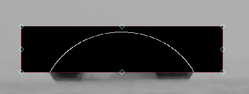
10.3.2 Binary Thresholding
Binary thresholding is the process by which the software converts the image to black and white to enable further analysis. In images with low contrast, Canny edge detection may be unable to find the edges of a droplet due to a low lightness gradient. Converting the image from greyscale to black and white using binary thresholding will result in distinct edges, enabling edge detection to work. Figure 10.8 shows the effect of binary thresholding when the ‘Binary Thresholding’ option has been toggled in the main viewer.
10.4 Pendant Drop Fitting
An optical tensiometer is a tool for measuring the surface tension of a liquid. The surface tension of a liquid determines how it changes shape under gravity, and thus the shape of a droplet as it hangs off a needle tip. Figure 8.6 shows a droplet attached to the end of a syringe needle. The top of the droplet is elongated, as the droplet deforms under its own weight. If the density and volume of the droplet is known, then its shape can be used to determine its surface tension.
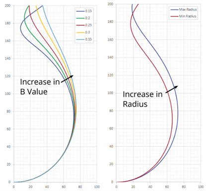
The fit has two main variables: droplet radius and B (a fitting constant). Figure 10.10 shows the effect that both the fitting constant and the radius have on a simulated droplet. The B value changes how a droplet shape deviates from a circle. The higher the value of B, the more deformed the droplet becomes due to gravity. Droplets with low surface tension are more deformed by gravity, so increasing B will give a lower surface tension in the droplet fit.
Changing the radius does not alter shape of the droplet like changing B does, however it changes the scale of the droplet. If a droplet’s volume is increased by its radius, it will deform more under the increased gravity. If two droplets have the same shape but different sizes, the larger droplet must therefore have a higher surface tension to retain the same shape with a higher volume. This means that increasing the simulated droplet radius will increase the surface tension.
The software iterates through value of radius and B to create many different simulated droplets. It then compares the simulated droplets with the detected edge of the droplet in the region of interest. The simulated fit that most closely matches the detected edge is chosen as the ‘real’ droplet. The difference between the simulated edge and the detected edge is the root mean squared error (RMSE). This is displayed when a measurement is performed and can be used as an indicator of how closely the simulated droplet matched the detected edge.
11. Miscellaneous
11.1 Theme
The software supports two themes which can be clicking the ‘Toggle Theme’ icon in the ‘View’ menu.
12. Troubleshooting
Before we send you your system, we run extensive tests to verify that it is stable and working. However, sometimes you may have issues connecting to and using the system. Most of the issues that may arise will be detailed here. If you encounter any problems, please contact Ossila.
Table 12.1 Troubleshooting guidlines for the Ossila Contact Angle Goniometer
| Problem | Possible Cause | Action |
|---|---|---|
| Backlight does not turn on. | The power supply may not be connected properly. | Ensure the system is firmly plugged into the power supply, and that the plug is connected to both the adapter and a working power socket. |
| The power supply adapter has a fault. | Contact Ossila for a replacement power supply adapter. | |
| Software does not start. | The wrong version of Windows is installed on the computer. | Install the software on a computer with Windows 10. |
| The software has not installed properly. | Try reinstalling the software. | |
| Cannot detect the camera. | The USB cable may not be connected properly. | Ensure the USB cable is firmly plugged in at both ends. |
| The USB cable may not be connected to a working USB port. | Try connecting the system to a different USB port on the computer. | |
| The USB cable is defective. | Try using a different USB cable and contact Ossila if necessary. | |
| Camera not responsive. | The camera connection has timed out. | Click the ‘Refresh Camera’ icon in ‘Tools’. |
| The USB connection has failed. | Try disconnecting and reconnecting the USB cable. |