Optical Spectrometer User Manual
Contents
- Overview
- EU Declaration of Conformity (DoC)
- Safety
- Requirements
- Unpacking
- Specifications
- Installation
- Device Overview
- Ossila Spectrometer Software
- Connecting a Device
- Window Layout
- Measurement Modes
- Trigger Modes
- Calibration
- Peak Finding Parameters
- Saving and Loading
- Example: Taking an Absorption Spectrum
- Offset and Gain Adjustment
- Sources of Noise
- Command Library
- Example Code
- Maintenance
- Troubleshooting
- Related Products
Optical Spectrometer

- Wide Spectral Range
- USB Powered
- Compact and Affordable
Available Now £1250
1. Overview
The Ossila USB powered Optical Spectrometer has been designed to simplify the optical characterisation of thin films, solutions, nanocrystals, photonic structures, and more. A compact enclosure combines with powerful electronics to deliver a fast, reliable, and cost-effective device. Take a measurement with a single click of a button with our free and intuitive spectroscopy software, or fully integrate it into your workflow through the use of a simple command library that gives you complete control over the system.

Key features:
- Wide spectral range (320 nm – 1050 nm)
- High resolution 16-bit ADC
- Integration time from 50 µs to 10 s
- Precision, compact enclosure
- USB-powered with USB type-C connection
- Powerful Arm Cortex M4 processor
- Up to 100 frames per second readout
- Internal and external trigger modes
- Rolling integration mode
- Use with our free software or interface through simple serial commands
- External shutter trigger
- 2 general purpose digital output pins
2. EU Declaration of Conformity (DoC)
We
Company Name: Ossila BV
Postal Address: Biopartner 3 Building, Galileiweg 8
Postcode: 2333 BD Leiden
Country: The Netherlands
Telephone Number: +31 (0)718 081020
Email Address: info@ossila.com
declare that the DoC is issued under our sole responsibility and belongs to the following product:
Product: Spectrometer (G2001A1)
Serial Number: G2001A1 - xxxx
Object of Declaration
Spectrometer (G2001A1)
The object of declaration described above is in conformity with the relevant Union harmonisation legislation:
EMC Directive 2014/30/EU
RoHS Directive 2011/65/EU
Signed:

Name: Dr James Kingsley
Place: Leiden
Date: 16/11/2021
| Декларация | за съответствие на ЕС |
|---|---|
| Производител | Ossila BV, Biopartner 3 building, Galileiweg 8, 2333 BD Leiden, NL. |
| Декларира с цялата си отговорност, че посоченото оборудване съответства на приложимото законодателство на ЕС за хармонизиране, посочено на предходната(-ите) страница(-и) на настоящия документ. | |
| [Čeština] | Prohlášení o shodě EU |
|---|---|
| Výrobce | Ossila BV, Biopartner 3 building, Galileiweg 8, 2333 BD Leiden, NL. |
| Prohlašujeme na vlastní odpovědnost, že uvedené zařízeni je v souladu s příslušnými harmonizačními předpisy EU uvedenými na předchozích stranách tohoto dokumentu. | |
| [Dansk] | EU-overensstemme lseserklærin g |
|---|---|
| Producent | Ossila BV, Biopartner 3 building, Galileiweg 8, 2333 BD Leiden, NL. |
| Erklærer herved, at vi alene er ansvarlige for, at det nævnte udstyr er i overensstemmelse med den relevante EUharmoniseringslovgivning, der er anført på den/de foregående side(r) i dette dokument. | |
| [Deutsch] | EU-Konformitätserklärung |
|---|---|
| Hersteller | Ossila BV, Biopartner 3 building, Galileiweg 8, 2333 BD Leiden, NL. |
| Wir erklären in alleiniger Verantwortung, dass das aufgeführte Gerät konform mit der relevanten EUHarmonisierungsgesetzgebung auf den vorangegangenen Seiten dieses Dokuments ist. | |
| [Eesti keel] | ELi vastavusavaldus |
|---|---|
| Tootja | Ossila BV, Biopartner 3 building, Galileiweg 8, 2333 BD Leiden, NL. |
| Kinnitame oma ainuvastutusel, et loetletud seadmed on kooskõlas antud dokumendi eelmisel lehelküljel / eelmistel lehekülgedel ära toodud asjaomaste ELi ühtlustamise õigusaktidega. | |
| [Ελληνικά] | Δήλωση πιστότητας ΕΕ |
|---|---|
| Κατασκευαστής | Ossila BV, Biopartner 3 building, Galileiweg 8, 2333 BD Leiden, NL. |
| Δηλώνουμε υπεύθυνα όn ο αναφερόμενος εξοπλισμός συμμορφώνεται με τη σχεnκή νομοθεσία εναρμόνισης της ΕΕ που υπάρχει σnς προηγούμενες σελίδες του παρόντος εγγράφου. | |
| [Español] | Declaración de conformidad UE |
|---|---|
| Fabricante | Ossila BV, Biopartner 3 building, Galileiweg 8, 2333 BD Leiden, NL. |
| Declaramos bajo nuestra única responsabilidad que el siguiente producto se ajusta a la pertinente legislación de armonización de la UE enumerada en las páginas anteriores de este documento. | |
| [Français] | Déclaration de conformité UE |
|---|---|
| Fabricant | Ossila BV, Biopartner 3 building, Galileiweg 8, 2333 BD Leiden, NL. |
| Déclarons sous notre seule responsabilité que le matériel mentionné est conforme à la législation en vigueur de l'UE présentée sur la/les page(s) précédente(s) de ce document. | |
| [Hrvatski] | E.U izjava o sukladnosti |
|---|---|
| Proizvođač | Ossila BV, Biopartner 3 building, Galileiweg 8, 2333 BD Leiden, NL. |
| Izjavljujemo na vlastitu odgovornost da je navedena oprema sukladna s mjerodavnim zakonodavstvom EU-a o usklađivanju koje je navedeno na prethodnoj(nim) stranici(ama) ovoga dokumenta. | |
| [Italiano] | Dichiarazione di conformità UE |
|---|---|
| Produttore | Ossila BV, Biopartner 3 building, Galileiweg 8, 2333 BD Leiden, NL. |
| Si dichiara sotto la propria personale responsabilità che l'apparecchiatura in elenco è conforme alla normativa di armonizzazione UE rilevante indicata nelle pagine precedenti del presente documento. | |
| [Latviešu] | ES atbils tības deklarācija |
|---|---|
| Ražotājs | Ossila BV, Biopartner 3 building, Galileiweg 8, 2333 BD Leiden, NL. |
| Ar pilnu atbilclību paziņojam, ka uzskaitītais aprīkojums atbilst attiecīgajiem ES saskaņošanas tiesību aktiem, kas minēti iepriekšējās šī dokumenta lapās. | |
| [Lietuvių k.] | ES atitikties deklaracija |
|---|---|
| Gamintojas | Ossila BV, Biopartner 3 building, Galileiweg 8, 2333 BD Leiden, NL. |
| atsakingai pareiškia, kad išvardinta įranga atitinka aktualius ES harmonizavimo teisės aktus, nurodytus ankstesniuose šio dokumento | |
| [Magyar] | EU-s megfelelőségi nyilatkozat |
|---|---|
| Gyártó | Ossila BV, Biopartner 3 building, Galileiweg 8, 2333 BD Leiden, NL. |
| Kizárólagos felelösségünk mellett kijelentjük, hogy a felsorolt eszköz megfelel az ezen dokumentum előző oldalán/oldalain található EU-s összehangolt jogszabályok vonatkozó rendelkezéseinek. | |
| [Nederlands] | EU-Conformiteitsverklaring |
|---|---|
| Fabrikant | Ossila BV, Biopartner 3 building, Galileiweg 8, 2333 BD Leiden, NL. |
| Verklaart onder onze uitsluitende verantwoordelijkheid dat de vermelde apparatuur in overeenstemming is met de relevante harmonisatiewetgeving van de EU op de vorige pagina('s) van dit document. | |
| [Norsk] | EU-samsvarserklæ ring |
|---|---|
| Produsent | Ossila BV, Biopartner 3 building, Galileiweg 8, 2333 BD Leiden, NL. |
| Erklærer under vårt eneansvar at utstyret oppført er i overholdelse med relevant EU-harmoniseringslavverk som står på de(n) forrige siden(e) i dette dokumentet. | |
| [Polski] | Deklaracja zgodności Unii Europejskiej |
|---|---|
| Producent | Ossila BV, Biopartner 3 building, Galileiweg 8, 2333 BD Leiden, NL. |
| Oświadczamy na własną odpowiedzialność, że podane urządzenie jest zgodne ze stosownymi przepisami harmonizacyjnymi Unii Europejskiej, które przedstawiono na poprzednich stronach niniejszego dokumentu. | |
| [Por tuguês] | Declaração de Conformidade UE |
|---|---|
| Fabricante | Ossila BV, Biopartner 3 building, Galileiweg 8, 2333 BD Leiden, NL. |
| Declara sob sua exclusiva responsabilidade que o equipamento indicado está em conformidade com a legislação de harmonização relevante da UE mencionada na(s) página(s) anterior(es) deste documento. | |
| [Română] | Declaraţie de conformitate UE |
|---|---|
| Producător | Ossila BV, Biopartner 3 building, Galileiweg 8, 2333 BD Leiden, NL. |
| Declară pe proprie răspundere că echipamentul prezentat este în conformitate cu prevederile legislaţiei UE de armonizare aplicabile prezentate la pagina/paginile anterioare a/ale acestui document. | |
| [Slovensky] | Vyhlásenie o zhode pre EÚ |
|---|---|
| Výrobca | Ossila BV, Biopartner 3 building, Galileiweg 8, 2333 BD Leiden, NL. |
| Na vlastnú zodpovednosť prehlasuje, že uvedené zariadenie je v súlade s príslušnými právnymi predpismi EÚ o harmonizácii uvedenými na predchádzajúcich stranách tohto dokumentu. | |
| [Slovenščina] | Izjava EU o skladnosti |
|---|---|
| Proizvajalec | Ossila BV, Biopartner 3 building, Galileiweg 8, 2333 BD Leiden, NL. |
| s polno odgovornostjo izjavlja, da je navedena oprema skladna z veljavno uskladitveno zakonodajo EU, navedeno na prejšnji strani/prejšnjih straneh tega dokumenta. | |
| [Suomi] | EU-vaatimustenm ukaisuusvakuutus |
|---|---|
| Valmistaja | Ossila BV, Biopartner 3 building, Galileiweg 8, 2333 BD Leiden, NL. |
| Vakuutamme täten olevamme yksin vastuussa siitä, että tässä asiakirjassa luetellut laitteet ovat tämän asiakirjan sivuilla edellisillä sivuilla kuvattujen olennaisten yhdenmukaistamista koskevien EU-säädösten vaatimusten mukaisia. | |
| [Svenska] | EU-försäkran om överensstämmelse |
|---|---|
| Tillverkare | Ossila BV, Biopartner 3 building, Galileiweg 8, 2333 BD Leiden, NL. |
| Vi intygar härmed att den utrustning som förtecknas överensstämmer med relevanta förordningar gällande EUharmonisering som fmns på föregående | |
3. Safety
3.1 Warning
- Do NOT connect a power supply to the Spectrometer’s USB port. It should only be connected to the USB port of a PC via a USB type-C cable.
- The maximum input/output voltage of the Spectrometer’s digital pins is 5V.
3.2 Use of Equipment
The Ossila Spectrometer is designed to be used as instructed. It is intended for use under the following conditions:
- Indoors in a laboratory environment (pollution degree 2).
- Altitudes up to 2000 m.
- Temperatures of 5°C to 40°C; maximum relative humidity of 80% up to 31°C.
3.3 Servicing
If servicing is required, please return the unit to Ossila Ltd. The warranty will be invalidated if:
- Modification or service has taken place by anyone other than an Ossila engineer.
- The Unit has been subjected to chemical damage through improper use.
- The Unit has been operated outside the usage parameters stated in the user documentation associated with the Unit.
- The Unit has been rendered inoperable through accident, misuse, contamination, improper maintenance, modification, or other external causes.
4. Requirements
The minimum computer specifications for the Ossila Spectrometer software are provided in Table 4.1.
Table 4.1. Ossila Spectrometer software requirements.
| Operating Systems | Windows 10 |
|---|---|
| CPU | Dual Core 2.0 GHz |
| RAM | 2 GB |
| Available Hard Drive Space | 300 MB |
| Monitor Resolution | 1280 x 960 |
| Connectivity | USB 2.0 |
5. Unpacking
5.1 Packing List
The standard items included with the Ossila Spectrometer are:
- The Ossila Spectrometer.
- USB type-A to type-C cable.
- USB memory stick pre-loaded with the user manual, quality control data, and software installer.


5.2 Damage Inspection
Examine the components for evidence of shipping damage. If damage has occurred, please contact Ossila directly for further action. The shipping packaging will come with a shock indicator to show if there has been any mishandling of the package during transportation.
6. Specifications
The Ossila Spectrometer technical specifications are shown in Table 6.1.
Table 6.1. Spectrometer specifications.
| Dimensions |
Width: 78 mm Height: 38 mm Depth: 78 mm |
|---|---|
| Weight | 150 g |
| Wavelength range | 320 nm - 1050 nm |
| Grating blaze wavelength | 500 nm |
| Resolution (FWHM) | 2.5 nm |
| Optical input | SMA 905 fibre or free space |
| Entrance slit width | 25 µm |
| Connection type | USB type-C |
| Communication protocol | Serial-over-USB |
| Dark noise* | < 50 counts |
| Signal-to-noise ratio | > 500:1 |
| Detector type / pixels | CCD / 1600 |
| Analog-to-digital converter | 16-bit, 500 kSPS |
| Data transfer speed* | Up to 100 FPS (PC dependant) |
| Stray light | < 0.2 % |
* Measured at 50 µs integration time, no spectral averaging.
7. Installation
- Install the Ossila Spectrometer software on your PC.
- Run the file ‘Ossila-Spectrometer-Installer-vX-X-X-X.exe’ on the USB memory stick provided.
- Follow the on-screen instructions to install the software.
- Connect the unit to your PC using the provided USB type-A to USB type-C cable.
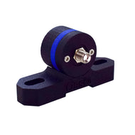
8. Device Overview


- Spectrometer entrance. The spectrometer features a 25 µm entrance slit with a UV-silica window to prevent contamination of the optics chamber. The spectrometer can be either fibre coupled (SMA905) or free-space coupled.
- USB type-C receptacle. The spectrometer receives power and communicates with the PC through a USB cable.
- Power LED. The LED turns on when the spectrometer electronics are active
- I/O expansion header. Used for functions including external/rolling triggers and shutter output.
8.1 I/O Expansion Header
The expansion header allows the spectrometer to interface with other devices using 5V signals. A wire jumper can be plugged into the header ports. The ports are labelled according to Figure 8.2. Note that there is an indentation next to port 1. Note that there is an indentation next to port 1.

Table 8.1. I/O expansion header descriptions.
| Port | Description | Direction |
|---|---|---|
| 1 | Ground. Connected to the system ground. Use this port to align ground levels between devices. | Output |
| 2 | External trigger. A 5V rising edge on this port will trigger an acquisition with the current device settings. | Input |
| 3 | Rolling shutter. A 5V rising edge on this pin will begin an integration, and a subsequent falling edge will end the integration (i.e., the integration time is the time the input remains high). The acquisition will be read out after the falling edge. | Input |
| 4 | Shutter fire. This port can be used to control an external shutter. It will be high (5V) during an acquisition, and at ground otherwise. Note that during continuous acquisition, this port will remain high (5V). | Output |
| 5 | Digital output 1. User controllable digital output. | Output |
| 6 | Digital output 2. User controllable digital output. | Output |
9. Ossila Spectrometer Software
9.1 Connecting a Device
When the software starts, the user will be presented with the device connection box. Any Ossila Spectrometer devices connected to the computer that are detected by the software will appear in the dropdown box.

Select the required device and press ‘Connect’. If a device is disconnected while the software is running, the software will attempt to reconnect automatically. If it is unable to reconnect, a warning message will appear followed by the device connection box. The connection window can also be opened from the toolbar or ‘System’ menu.

9.2 Window Layout
The Ossila Spectrometer software window is separated into areas indicated in Figure 9.2. The function of these areas are briefly outlined below.
9.2.1 Menu Bar
Access various features related to device and software settings.
(I) File
- Restart session – Clear all data from the program memory.
- Open – Open a saved spectrum. Multiple saved spectra can be imported at once.
- Save Checked Spectra – Save spectra that have been checked in the workspace to file.
- Toggle Autosave – Turn auto save on/off. When on, newly acquired spectra will automatically be saved to the autosave directory. The first time autosave is activated in a session, a prompt will appear to set the autosave directory. This can also be set or changed using Set Autosave Directory option.
- Set Autosave Directory – Set/change the directory to which spectra will be saved.
- Quit – Close the program
(II) System
- Connect – (Re)connect to a device.
- Reset Calibration – Return the wavelength calibration to factory setting.
- Open Command Window – Opens a window to communicate with the system directly through the serial command library. The available commands are given in Section 13.

(III) Experiment
- Continuous Data Acquisition – Begin continuous measurement.
- Single Shot Data Acquisition – Take single measurement.
- Stop Data Acquisition – Stop current measurement.
- Get Background – Take a background spectrum.
- Get Reference - Take a reference spectrum. Note that a background spectrum must be taken first.
(IV) Tools
- Calibrate Using Selected Spectrum – Transfer the selected spectrum into the calibration window. See Section 9.5 for details.
- Find Peak Parameters – Open dialog box to set parameters related to peak detection. See Section 9.6 for details.
(V) View
- Toggle Dark Theme – Change the software theme to dark mode. Useful for minimising computer screen light for sensitive measurements.
- Show Frames Per Second – If enabled, the rate at which spectra are being read from the spectrometer is shown in the status bar. Additional processing of spectra, such as peak detection, can reduce the frame rate.
- Scroll to Most Recent Spectrum – When enabled, the workspace will automatically scroll to a newly recorded spectrum. When disabled, the workspace can be scrolled (if enough spectra are present in the workspace) so that previously recorded spectra can be check/unchecked while an acquisition is in progress.


9.2.2 Quick Access Buttons and Acquisition Settings
Buttons to access common features. Hover the mouse cursor over the button to display a tooltip. The buttons have the following functions:
|
|
Open previously saved spectra. |
|
|
Save checked spectra. |
|
|
Open device connection menu. |
|
|
Continuous Data Acquisition. |
|
|
Single Shot Data Acquisition. |
|
|
Stop Data Acquisition. |
|
|
Pin new spectra. This will keep all newly recorded spectra in the workspace. |
|
|
Take a background spectrum. |
|
|
Take a reference spectrum. Note that a background spectrum must be taken first. |
Commonly adjusted acquisition settings are also available in this area.
(I) Integration Time
Sets the integration time of the acquisition. The allowed range is from 50 µs to 10 s (0.05 ms to 10000 ms).
(II) Delay
Introduces a delay between successive measurements. A delay of 0 seconds will result in the spectrometer taking acquisitions as quickly as possible. The maximum allowed delay is 99.99 seconds. This value is ignored in ‘external trigger’ and ‘rolling integration’ modes.
(III) Accumulation
Sets the number of successive spectra to sum together. The maximum allowed value is 20.
(IV) Averaging
Sets the number of successive spectra that are used to calculate a mean value. The maximum allowed value is 99.
9.2.3 Measurement Settings
(I) Trigger
There are 3 trigger modes available: internal trigger, external trigger and rolling integration. See Section 9.4 for a description of these modes.
(II) Measurement
There are 3 measurement types available. See section Section 9.3 for a full description of these.
9.2.4 Plot properties
Used to customise the appearance of the plot(s) and enable/disable peak detection features.
(I) Peaks
Displays detected peak positions on the currently selected spectrum.
(II) Widths
Displays detected peak widths on the currently selected spectrum.
(III) Autorange
Automatically scales the y-axis to display the entirety of the currently selected spectrum.
(IV) Spectrum Colour
Shows a colour palette fill under the currently selected spectrum, representing an approximation of the colour of light at each wavelength.
(V) Grid
Adds a grid to the plot background.
9.2.5 Cursor
Displays the current cursor (wavelength and intensity) position on the plot.
9.2.6 Smoothing
Whilst smoothing is checked, a Savitzky-Golay smoothing filter will be applied to the data displayed in the plot window. The parameters of the filter can be selected using the Data Points and Polynomial boxes.
(I) Data Points
The number of data points to use when calculating the polynomial fit for each smoothed data point.
(II) Polynomial
The order of the polynomial to use for fitting each data point. This must be less than the value of Data Points.
9.2.7 Spectra Workspace
The current spectrum and any pinned spectra will be visible in this workspace. New spectra are unpinned by default (unless the ‘Pin new spectra’ button is active), meaning that subsequent spectra will overwrite the current spectra. To prevent the current spectrum from being overwritten in the workspace, click the ‘Keep Last Spectrum’ button while it is selected.
Spectra can be selected by clicking on their name (selection of multiple spectra is supported though use of the Shift and Ctrl keys on the keyboard). Selected spectra appear highlighed in blue and can be removed from the workspace using the ‘Delete Selected Spectra’ button. All spectra can be removed from the workspace with the ‘Clear All’ button.
Only checked spectra are visible on the plot. A checked spectra will have a tick in the checkbox next to it’s name. Individual spectra can be checked and unchecked by clicking on the checkbox. Multiple spectra can be checked by first selecting them, and them using the ‘Check All Selected’ button. All spectra in the workspace can be unchecked (i.e. the plot cleared) by using the ‘Uncheck All’ button.
9.2.8 Spectrum Properties
The Spectrum Properties box contains two tabs called ‘Spectrum’ and ‘Data’.
(I) Spectrum
The ‘Spectrum’ tab contains details of the currently selected spectrum (or last selected spectrum in the case that multiple spectra are selected). Editable fields are the spectrum name, comments, and the colour the spectrum appears in the plot. Information fields include the time it was taken, the device on which it was recorded, and the measurement parameters that were used.
(II) Data
The ‘Data’ tab shows the numerical data for the selected spectrum. If the spectrum was taken in a measurement type that requires a background/reference spectrum, the background/reference data will also be shown here. The ‘intensity’ field shows the numerical value after processing, for example it will show absorbance data if the measurement mode is Absorption. This does not update while taking continuous measurements.
9.2.9 Status Bar
Shows the most recently completed action, the device status and whether background and reference spectra have been recorded. The frames-per-second will also be shown here if enabled in the Tools menu.
9.2.10 Plot Window
All checked spectra in the Spectra Workspace are plotted in this area. Navigation (zooming and panning) is performed with a mouse. There are 2 options for for the mouse interface behaviour: 1-button mouse and 3-button mouse. This can be selected by right-clicking in the plot area and selecting ‘Mouse Mode’ from the menu.
(I) 3-Button Mode (Default)
- Left/middle click and drag – pan the axes.
- Scroll wheel – zoom plot (scale the axes) centred on the cursor location.
- Right click and drag – scale the axes (left-right movement zooms the x-axis, up-down movement zooms the y-axis).
(II) 1-Button Mode
- Left/middle click and drag – draw region of interest, when released the plot will zoom to the selected region.
- Scroll wheel – zoom plot (scale the axes) centred on the cursor location.
- Right click and drag – scale the axes (left-right movement zooms the x-axis, up-down movement zooms the y-axis).
In both modes a specific axis can be controlled by using these controls on the axis labels.
9.3 Measurement Modes
The Ossila Spectrometer software can perform measurements in the following modes:
(I) Intensity
The raw output from the analogue-to-digital converter is displayed. This can take values between 0 and 65534. Even in complete darkness, the spectrum will have a dark count.
(II) Intensity (Background Corrected)
The output is background corrected. The user must first take a background spectrum, which will be subtracted from any subsequent plots taken in this mode.
(III) Intensity (Sensitivity Corrected)
The spectrum is corrected for the spectral response of the system. The system spectral response is only measured between 350 nm and 1050 nm. Any data points out of this range will use an interpolated correction which may not be accurate. A background spectrum must be taken before using this mode.
(IV) Transmission/Reflection
The output is both background corrected and scaled (divided) by a reference spectrum. A background and reference spectrum must be present to select this measurement mode.
(V) Absorption
Signal is calculated according to log10( 1 / transmission). A background and reference spectrum must be present to select this measurement mode.
Trigger Modes
The Ossila Spectrometer has three trigger modes that can be selected from the ‘Trigger’ dropdown box in the Measurement Settings.
(I) Internal Trigger
The start and end times of acquisitions are handled by the spectrometer. The time spent collecting a signal is determined by the integration time.
(II) External Trigger
A 5V rising edge on the external trigger port will begin the acquisition. The time spent collecting a signal is determined by the integration time.
(III) Rolling Integration
A 5V rising edge on the rolling integration port will begin the acquisition. The acquisition will end when the voltage at the port returns to 0V. If the voltage changes from 5V to 0V within the debounce time, the trigger will not be registered.
Note that a trigger will be ignored if it arrives either while there is an acquisition in progress or while the spectrum is being sent.
Debounce Time
The external trigger and rolling integration modes have a user settable debounce time. A longer debounce time will help to eliminate electrical chatter often found when using mechanical switches. However, it will increase the time between the signal being detected and the operation being implemented. If using a transistor-to-transistor logic (TTL ) signal to control these functions, the debounce time can be reduced to minimise this delay. The debounce time can be set using the <debounce:value> command in the command window. Note that even with a debounce time of 0 µs, it will take up to 1.5 µs for the system to register the trigger.
CCD Flush
The CCD flush settings will also affect the delay between receiving a trigger and the acquisition starting. The CCD flush before reading can be disabled to minimise this delay, however this should only be done if an external shutter is used and may result in higher background counts. With the flush enabled, the delay between detecting the trigger and starting the acquisition is approximately 40 µs. With the flush disabled this delay is reduced to 15 µs.
9.5 Calibration
The Ossila USB Spectrometer is factory calibrated for wavelength. Over time, it may be necessary to recalibrate the system. This can be performed by the user. The factory calibration is permanently stored in the system memory, so any user calibration can be reverted to factory calibration if required. The procedure for calibrating the wavelength is given below.
- Record a spectrum, ideally one that has distinctive features at known wavelengths. In this example a compact-fluorescent light (CFL) is used to calibrate the system over the visible part of the spectrum.

- Select the spectrum in the workspace (highlighted blue) and select ‘Calibrate Using Selected Spectrum’ from the Tools menu. The calibration window will open with the selected spectrum visible.

- The calibration procedure will map pixel numbers to wavelength using a polynomial fit. Hover the mouse cursor over a feature to identify the pixel number and enter this into the ‘Pixel’ column. Enter the wavelength of this feature in the ‘Wavelength (nm)’ column. More rows can be added, or current rows removed using the ‘Add’ and ‘Delete’ buttons respectively. The graph can be zoomed and scrolled in the same way as the main window to help identify the pixels. Highlighting a box in the ‘Pixel’ column and then double clicking on the graph will automatically populate the box with the curser location. At least 2 points should be used for calibration, with more points typically giving a better fit. The pixel numbers and wavelengths do not need to be in ascending order; however, the data pairs must be monotonic (increasing pixel number results in increasing wavelength).
- Click the calibrate button. A progress bar will appear in the top left of the window. If the calibration is successful, a dialog box will appear confirming whether to close the calibration window. The new calibration is now saved on the device. Any new spectra will be displayed with the new wavelength calibration.
The calibration can be reset to the factory values by opening the command window from the System toolbar and sending <resetwavcal:1> to the device.
9.6 Peak Finding Parameters
The software can identify up to 20 peaks in a spectrum. This feature is enabled using the check boxes in the Plot Properties menu. Enabling ‘Peaks’ will display the peak positions next to the identified peaks, while ‘Widths’ will show the full-width-half-maximum of the peak. Note that enabling either or both peak finding functions may reduce the data rate.
The peak finding parameters define the conditions required for a peak to be identified. They can be accessed by selecting ‘Find Peak Parameters’ from the Tools menu. A peak should fulfil all the parameters in order to be identified.

The meanings of the parameters are as follows:
- Height – The minimum height of a peak as measured from 0.
- Threshold – The minimum vertical difference between the maximum point and the neighbouring points. This is generally used for identifying very narrow peaks and is normally be set to 0.
- Prominence – The vertical separation between the peak and its highest minimum contour, i.e., for a symmetrical peak it is the vertical distance between the summit and the base, for a non-symmetrical peak it is the vertical distance between the summit and its highest bottom edge.
- Width – The minimum width (in pixels) of a peak.
If the set parameters result in the identification of more than 20 peaks, a warning message will appear, and the peak finding functions will be disabled.
9.7 Saving and Loading
Spectra can be saved either manually or automatically. To manually save spectra:
- For the spectra you want to save check the tick-box to the left of the spectra name.
- Open the File menu and select ‘Save Checked Spectra’.
- In the dialog box, navigate to the directory you want to save to.
- Click the ‘Save’ button. The file name will be the spectrum name, suffixed with the timestamp of the acquisition.
Each spectrum is saved as a separate comma-separated variable (CSV) file. This can be opened by most spreadsheet, graphing, or text-editing software. The file structure consists of a header which contains the device and acquisition details, and four columns containing the wavelength (in nanometres), intensity, background and reference. If no background or reference spectra were used in the acquisition, these columns will be empty. The ‘intensity’ column shows the numerical value after processing, for example, it will show absorbance data if the measurement mode is Absorption.
Spectra can be saved automatically by enabling the Autosave feature from the File menu. The first time the ‘Toggle Autosave’ feature is activated, a dialog box will show to select a directory into which to save spectra. This directory can be changed later using the ‘Set Autosave Folder’ feature, also in the Tools menu. Only spectra that are kept in the workspace will be saved, so it is necessary to press the ‘Keep All New Spectra’ button on the quick access bar to save every new spectrum.

Previously saved spectra can be loaded into the software using the ‘Open’ feature in the File menu. A file explorer dialog box will open, and multiple files can be selected for importation.
10. Example: Taking an absorption spectrum
Here we will give the process of recording an example absorption spectrum from a thin film.
First, connect the spectrometer to a PC and open the Ossila Spectrometer Software. We suggest allowing 30 minutes for the temperature of the electronics to stabilize before taking measurements.
Next, set up the experiment. Absorption measurements require a sample to be placed in between a light source and the spectrometer. In this example we will use the Ossila Broadband White Light Source and the Ossila Transmission Holder (both sold separately). However, any light source that emits over the range of the required absorption spectrum would be sufficient, and any method of fixing the sample between the light source and the spectrometer is acceptable.

Arrange the spectrometer, sample holder and light source as shown in Figure 10.1. It is good practice to perform these measurements in a darkened room (or to cover the entire setup) to minimise any external factors in the measurement.
Now we will identify an appropriate integration time for the measurement. Ensure that the sample holder is empty and turn the light source on. Run a continuous acquisition and adjust the integration time until the maximum signal reads approximately 50000 counts. Note that the CCD response becomes non-linear above approximately 60,000 counts which may affect measurements. In this case, an integration time of 30 ms is sufficient.
Absorption measurements are particularly susceptible to noise as they involve the combination of 3 different spectra (background, reference and signal). Noise in the individual spectra is amplified when they are combined. To reduce the effect of noise, we can use the Averaging function. Here, we will set it to average 50 spectra. Now, turn the light source off, and take a background spectrum.
Turn the light source on and take a reference spectrum. If you are measuring the absorption of a thin film on a substrate (e.g., glass), you should place a blank substrate in the sample position while taking the reference measurement. This will ensure any absorption contribution by the substrate is excluded from the measurement. Note the wavelength range over which the light source emits – this is the range over which the absorption measurement is valid. Any data outside of this range will be meaningless.

Now, carefully load the sample into position. The alignment of the apparatus must not change in between taking the reference spectrum and the data. If using optical fibres, do not rearrange their positions at this point.

Change the Measurement Type to absorption. Uncheck the background and reference spectra in the workspace. Take a Single Shot measurement. Absorption measurements generally have a value between 0 and 4, so the y-axis needs to be scaled to see the spectrum. This can be done by right-clicking on the plot and selecting ‘View All’. The absorption spectrum of the sample is shown in Figure 10.4. Note the data outside of the light source emission range (approximately 370 nm – 850 nm) appears extremely noisy. This is because you cannot calculate the absorption of light if there is no light to be absorbed, therefore this data should be discarded.

11. Offset and Gain Adjustment
The offset and gain are two parameters which determine how the analogue voltage from the CCD is conditioned before it arrives at the analogue-to-digital converter. The offset determines the baseline (i.e., non-background subtracted dark) signal counts, and the gain scales the CCD output. Both values are controlled by 10-bit digital potentiometers and can be adjusted by the user between the values of 0 and 1023. The offset is determined individually for each spectrometer during the calibration process. The default gain is set to the midrange value of 512. It should not be necessary to change the gain under normal operation, but the user may want to adjust the offset.
The output baseline voltage of the CCD is dependent on temperature. At low temperatures, the baseline may drop below the measurement floor of the ADC. In this situation, the offset should be reduced (reducing the offset increases the baseline position). This is evident as the dark signal will be approximately 400 counts (this will vary slightly from device to device) and the RMS noise on a dark signal will be close to 1 count. Conversely, at high temperatures the system may display a high baseline signal. Increasing the offset will allow a higher dynamic range to be achieved.
The effect of too low and too high a baseline is shown in Figure 11.1. The system is set up such that it would not need adjusting if used within the temperature range 10°C – 30°C.

The offset and gain values can be adjusted from within the Ossila Spectrometer Software by opening the command window from the System menu in the toolbar. The <offset?> and <gain?> commands can be used to query the current offset, and the <offset:value> and <gain:value> commands can be used to set new values. The default values can be restored by sending <resetscale:1>.


12. Sources of Noise
12.1 Thermal Noise
A significant source of noise from a CCD is thermal noise. It is random in nature and increases with both integration time and temperature. Figure 12.1 shows dark spectra taken with 3 different integration times: 50 µs (green), 500 ms (blue) and 5 s (red). For low and moderate integration times (< 1s), thermal noise is dominant. Thermal noise is not affected by subtracting a background spectrum (due to its randomness) but can be reduced by averaging consecutive spectra.

A periodic signal becomes visible for long integration times. This is not noise as such but is caused by different sensitivities of the pixels. It can therefore be removed by subtracting a background signal. Figure 12.2 shows an uncorrected and background corrected dark signal at 5 s integration time.

12.2 Periodic Noise
A second type of periodic signal can be visible at short integration times (< 6ms). It is normally obscured by thermal noise, however averaging many spectra to suppress the thermal noise, the signal becomes visible. This is due to the internal operation of the CCD, in particular the electronic shutter which allows the system to perform short integrations. For a given integration time, the position and magnitude of this signal is fixed, so it too can be removed by performing a background subtraction. Figure 12.3 shows dark spectra taken with an integration time of 50 µs, averaged over 99 spectra without (red) and with (green) background correction.

It is good practice to use a background correction when performing sensitive measurements. Background and reference spectra should be remeasured if any of the acquisition settings are changed (i.e., integration time, accumulations or averaging).
15. Command Library
The Ossila Spectrometer communicates with a host computer through a serial command library. When connected to a PC, the system will appear as a COM port, to which the serial commands could be sent. This section describes the command protocol and lists the available commands.
13.1 Command Format
Commands should be sent to the spectrometer in ASCII format, and responses from the spectrometer will also be in ASCII format, except for spectral data, which is sent as an unsigned 16-bit binary number.
All commands sent to the spectrometer have a start and end delimiter (‘<’ and ‘>’ respectively). Only commands enclosed by these delimiters will be acknowledged by the device. If any invalid commands are sent between delimiters, the system will return ‘<Invalid Command>’. Commands can be setting commands or query commands.
Setting commands have the format ‘<parameter:value>’, where ‘parameter’ is the setting to be changed, and value is the new value. The new value will be either a floating-point number, integer or boolean (0 or 1). Floating point numbers can be sent in scientific notation (e.g., 123e4 or 123E4). If a command requires an integer and a floating-point value is sent, the system will round the number down to an integer. If a value outside of the allowed range is given, it will be coerced into the allowed range. If a Boolean is required and a non-zero floating-point number (or integer other than 0 or 1) is sent, the system will interpret it as a ‘1’. If a setting command is successfully implemented, the system will echo back the command. The exception to this rule are the ‘<read:value>’, '<ext:value>' and '<roll:value>' commands, which will not be echoed back but will return a spectrum/spectra after the elapsed integration time.
Query commands have the format ‘<parameter?>’. These commands allow the user to find current system settings without modifying them. If a query command is successfully interpreted, the system will return ‘<parameter:value>’.
13.2 Setting Command List
| Command | Function | Expected Value |
|---|---|---|
| <itime:value> | Sets the integration time. | Integer between 50 and 10E6, representing the integration time in microseconds. |
| <read:value> | Begins measurement with current settings and returns spectrum/spectra. | Integer between 0 and 232-1 representing the number of spectra to take (0 is continuous reading). |
| <preflush:value> | Activates or deactivates flushing of the CCD before taking a measurement. | Integer. 0 to deactivate, 1 to activate once when an acquisition is started, 2 to activate before every scan. This is set to 2 by default and should only be changed by expert users. |
| <ext:value> | Activates external trigger mode. | Integer between 0 and 232-1 representing the number of times the system will respond to an external trigger before returning to an idle state (0 is unlimited). |
| <roll:value> | Activates rolling integration mode. | Integer between 0 and 232-1 representing the number of times the system will respond to an external trigger before returning to an idle state (0 is unlimited). |
| <polyX:value> | Sets the polynomial coefficient of order X for wavelength calibration. X can be an integer between 0 and 5. | Float. This can be stored with approximately 15 digits of precision. |
| <resetwavcal:value> | Restores the wavelength calibration polynomials to factory values. | Boolean. 0 has no effect, 1 restores the calibration. |
| <gain:value> | Sets the spectrum gain of the system. | Integer between 0 and 1023. Higher numbers give a larger positive gain. |
| <offset:value> | Sets the spectrum base level offset of the system. | Integer between 0 and 1023. Higher numbers give a larger negative offset. |
| <resetscale:value> | Restores the gain and offset to factory values. | Boolean. 0 has no effect, 1 restores the values. |
| <debounce:value> | Sets the debounce time for the trigger in external and rolling integration modes. | Integer between 0 and 1000000 representing the debounce time in microseconds. |
| <dXout:value> | Turns the digital output pin X on or off. X can be 1 or 2. | Boolean. 0 turns the output off, 1 turns the output on. The outputs are on by default when the system is connected. |
| <led:value> | Turns the power LED on/off. | Boolean. 0 turns LED off, 1 turns LED on. The LED is on by default when the system is connected. |
13.2.1 Interpreting the returned spectra
Spectral data returned from the spectrometer differs from all other data in that it is not in ASCII format. In order to maximise the speed of transmission, it is returned in binary 16-bit integer format. It also has unique start and end characters used to detect when the data has become corrupted between the device and the PC. A spectrum will consist of 1600 numbers between the values of 0 and 65353. These will be preceded by a value of 65354 and followed by a value of 65355. The spectrometer uses a 16-bit analogue-to-digital converter to digitise the optical signal. This can have output values between 0 and 65355, so in order to protect the starting and ending values, if any output in the data is above 65353, it is coerced down to this value. This has a negligible effect on the dynamic range of the system. An example of the spectral output of the system will therefore look like:

An example of reading a spectrum using the Python programming language is given in Section 14.
13.3 Query Command List
| Command | Function | Return |
|---|---|---|
| <itime?> | Returns the integration time. | <itime:value> where value is an integer between 10 and XXX representing the integration time in microseconds. |
| <preflush?> | Returns the state of the preflush function. | <preflush:value> where value is either 0 (off), 1 (flush on first acquisition) or 2 (flush on every acquisition). |
| <polyX?> | Returns the polynomial coefficient of order X for wavelength calibration. X can be an integer between 0 and 5. | <polyX:value> where value is the calibration polynomial coefficient of order X (returned as a float). |
| <gain?> | Returns the spectrum gain setting. | <gain:value> where value is the gain (returned as an integer between 0 and 1023). |
| <offset?> | Returns the spectrum offset setting. | <offset:value> where value is the offset (returned as an integer between 0 and 1023). |
| <debounce?> | Returns the debounce time for external and rolling integration triggers. | <debounce:value> where value is the debounce time in microseconds. |
| <dXout?> | Returns the state of digital output pin X. X can be 1 or 2. | <dXout:value> where value is 0 (off) or 1 (on). |
| <corr@X?> | Returns the relative system sensitivity at a wavelength of X, where X is and integer between 350 and 1050 representing the wavelength in nanometers. | <corr@X:value> where value is is a float representing the relative spectral sensitivity of the system at the wavelength of X nm. To apply a spectral correction, the correction values should be interpolated to give a spectral correction at a measured wavelength, and the measured intensity multiplied by the correction value. |
| <device?> | Returns the device name. | <Ossila Spectrometer> |
| <firmware?> | Returns the firmware number. | <firmware:value> where value is the firmware version (returned as a float). |
14. Example Code
The following code is written in the Python programming language and shows how to set up the device, and read and plot a spectrum.
# The PySerial library is required to communicate with the spectrometer
# Ensure that it is installed on your system before running this script
import serial

# We will use the NumPy library for dealing with the spectral data
import numpy as np

# matplotlib provides a simple way to plot data
import matplotlib.pyplot as plt

# Open a serial connection to the spectrometer
# In this example, the spectrometer is attached to COM port 18
# It is likely to be a different port on your computer
# In windows, you can see which port has been assigned in the Device Manager
s = serial.Serial('COM18')

# We can read the current integration time from the device using the <itime?> command
# The command needs to be converted into a byte array before being sent to the spectrometer
# This is done using the encode() function
s.write('<itime?>'.encode())

# The spectrometer will return the current integration time
# We can read its response with the .readline() function
# The decode() function is used to convert the response to a string
response = s.readline().decode()

# If we print the response, we will see <itime:xxx> where xxx is the integration time in microseconds
print(response)

# The integration time can be changed using the <itime:xxx> command
# Here we set it to 1 millisecond (1000 microseconds)
s.write('<itime:1000>'.encode())

# The spectrometer will echo back the command if successful
response = s.readline().decode()

# The response will be <itime:1000>
print(response)

# We can read a single spectrum from the device using the <read:1> command
s.write('<read:1>'.encode())

# There are 1600 pixels to read, each represented by a 16-bit integer
# There are also 2 start/stop values to read, also 16-bit each
# This gives the total number of bytes to read as (1600 + 2) * 2 = 3204
# We can specify how many bytes to read from the spectrometer using the read(bytes) function
# We will not decode the response this time as it is not in text data format
response = s.read(3204)

# Instead, we will put it into a NumPy array using the frombuffer() function
# We don't want the first 2 or last 2 bytes to be put into the array
# These are the start and stop numbers and not part of the data
spectrum = np.frombuffer(response[2:3202], dtype=np.uint16)

# We need the wavelengths to which the spectral data corresponds
# This can be read from the device using the <wavs?> command
s.write('<wavs?>'.encode())

# The response will be a list of 1600 numbers separated by commas
# These will be in text format so we can use the decode function
response = s.readline().decode()

# The wavelength data can be put into a NumPy array using the .fromstring() function
wavelength = np.fromstring(response, sep=',')

# The wavelength vs spectral data can now be plotted
plt.plot(wavelength, spectrum)

# Once the script is complete, close the interface to the spectrometer
s.close()
15. Maintenance
The Ossila Spectrometer is a sealed unit and should require no maintenance if used under the recommended conditions.
16. Troubleshooting
The most common issues that can arise will be detailed here, however, if you encounter any issue that isn’t detailed, then please don’t hesitate to contact us.
Table 16.1. Troubleshooting guidelines for the Ossila Optical Spectrometer.
| Problem | Possible cause | Action |
|---|---|---|
| Cannot connect to the system via USB | The USB cable may not be connected properly. | Ensure the USB cable is firmly plugged in at both ends. |
| The USB cable may not be connected to a working USB port. | Try connecting the system to a different USB port on the computer. If using a USB hub, try plugging the unit into a port directly on the PC. | |
| The USB cable is defective. | Try using a different USB cable. | |
| Software does not start | The wrong version of Windows is installed on the computer. | Install the software on a computer with Windows 10. |
| The software has not installed properly | Try reinstalling the software. |